3D Reentry Vehicle (ramC3d.pre)¶

Problem description¶

This example simulates the ballistic reentry of the RAMC module. The simulation is performed at an altitude of 61 km and an angle of attack of \(15^{\circ}\). The surface of RAMC is assumed to be made up of carbon material. Standard radiation equilibrium model is used to compute the surface temperature and then ablation of carbon from the surface is obtained. The fluid contains 7 air species and carbon atoms. The reactions and atomic data are given in the external text data file air7SpeciesAbCarbon.txt. Grid is generated using cubit.

This simulation can be performed using USimHS license.

Creating the run space¶

The 3D Reentry Vehicle example is accessed from within USimComposer by the following actions:

• Select the New from Template menu item in the File menu.
• In the resulting New from Template dialog, expand USimHS: Hypersonics.
• Select 3D Reentry Vehicle and press the Choose button.
• In the Choose a name for the new runspace dialog, press the Save button to create a copy of this example in your run area.
• Press the Save And Process Setup button in the upper right corner of the Editor pane.

The basic example variables are editable in the Editor pane of the Setup window. After any change is made, the Save and Process Setup button must be pressed again before a new run commences.

Input file features¶

The following parameters can be varied:

• GRIDFILE - name of grid file
• TEND - Simulation end time (seconds).
• NUMDUMPS - Number of data dumps during the simulation
• REACTIONS_ATOMIC_DATA - name of the file containing reactions and atomic data
• SPEED - free stream velocity
• AOA - angle of attack
• FREESTREAM_DENSITY - free stream density
• FREESTREAM_TEMPERATURE - free stream temperature
• SURFACE_EMISSIVITY - emissivity of the surface
• GAS_EMISSIVITY - emissivity of the hot gas in the vicinity of surface
• MW1_1 - molecular weight of species 1
• ABP01_1 - reference pressure of species 1
• ABDH1_1 - evaporation enthalpy of species 1
• ABT01_1 - reference temperature of species 1
• CFL_CONVECTIVE - CFL condition number for convective terms
• VISCOUS_DIFF_TIMESTEP_FACTOR - Factor to further decrease the internally computed time step based on kinematic viscosity
• THERMAL_DIFF_TIMESTEP_FACTOR - Factor to further decrease the internally computed time step based on thermal diffusicity
• BASEMENT_TEMPERATURE - least possible temperature in the domain (K).

The speed, angle of attack, free stream density, temperature are 7650 \(m/s\), \(15^{\circ}\), \(2.816^{-4} kg/m^3\), and 244.3 \(K\) respectively. Surface material is carbon. Note that the input file comes with an externally generated unstructured mesh using cubit.

Running the simulation¶

After performing the above actions, continue as follows:

• Proceed to the Run window as instructed by pressing the Run icon in the workflow panel.
• To run the simulation, click on the Run button in the upper right corner of the Logs and Output Files pane.

You will also see the engine log output in the Logs and Output Files pane. The run has completed when you see the output, “Engine completed successfully.”

Visualizing the results¶

After performing the above actions, continue as follows:

• Proceed to the Visualize window as instructed by pressing the Visualize icon in the workflow panel.

• Press the Open button to begin visualizing.

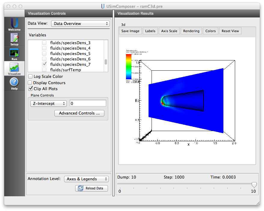
• Expand Scalar Data and click the check box for fluids/speciesDens_7.

• Check the Clip All Plots box and set the Z-intercept to 0.

• Drag the slider at the bottom of the Visualization Results pane to move through the simulation in time. The distribution at the end of the simulation is shown in Fig. 97.

  The conservative parameters density, three components of momentum, and energy can also be visualized using q_0,q_1,..,q_5 respectively.

Figure 98: Ablation species density on RAMC during reentry

Further experiments¶

• Change the flow speed: For example, decrease SPEED to 6000, keeping the other flow parameters unchanged. Follow the steps and complete the simulation.

• AOA: angle of attack may be changed to simulate trajectory maneuver.

• Altitude: Change in altitude can be simulated by varying the freestream density and temperature.

• Material: Change the surface material to say aluminum. The properties of aluminum MW1_1 = 27.0, ABP01_1 = 0.133, ABDH1_1 = 304807.868, ABT01_1 = 1351.9932. The name of the species in the reactionTableRhs block has to be updated to Al in the .pre file. In addition to these, the molecular weight and molecular diameter of species 7 have to be changed in the air7SpeciesAbCarbon.txt file. The change is given below:

  MOLECULARWEIGHT START

  SPECIES N2 N O2 O NO NO_p1 e Al

  28.0 14.0 32.0 16.0 30.0 30.0 5.5e-4 27.0

  MOLECULARWEIGHT END

  MOLECULARDIA START

  SPECIES N2 N O2 O NO NO_p1 e Al

  2.5e-10 2.0e-10 5.0e-10 2.0e-10 2.5e-10 2.5e-10 5.0e-13 2.7e-10

  MOLECULARDIA END

• Parallel: carry out the simulation on 2, 4, or 8 cores using the MPI options.