Verify EOS Table (verifyEOSTable.pre)¶

Problem description¶

This example verifies the result of interpolation and inverse interpolation from a SESAME equation-of-state (EOS) table. Fake data is provided for the purpose of this example. To use this example with the PROPACEOS reader, simply set INPUTFORMAT to 1. This replaces instances of sesameVariables with propaceosVariables and replaces 301energy and 301pressure with Eint and Ptot in the operations strings, respectively.

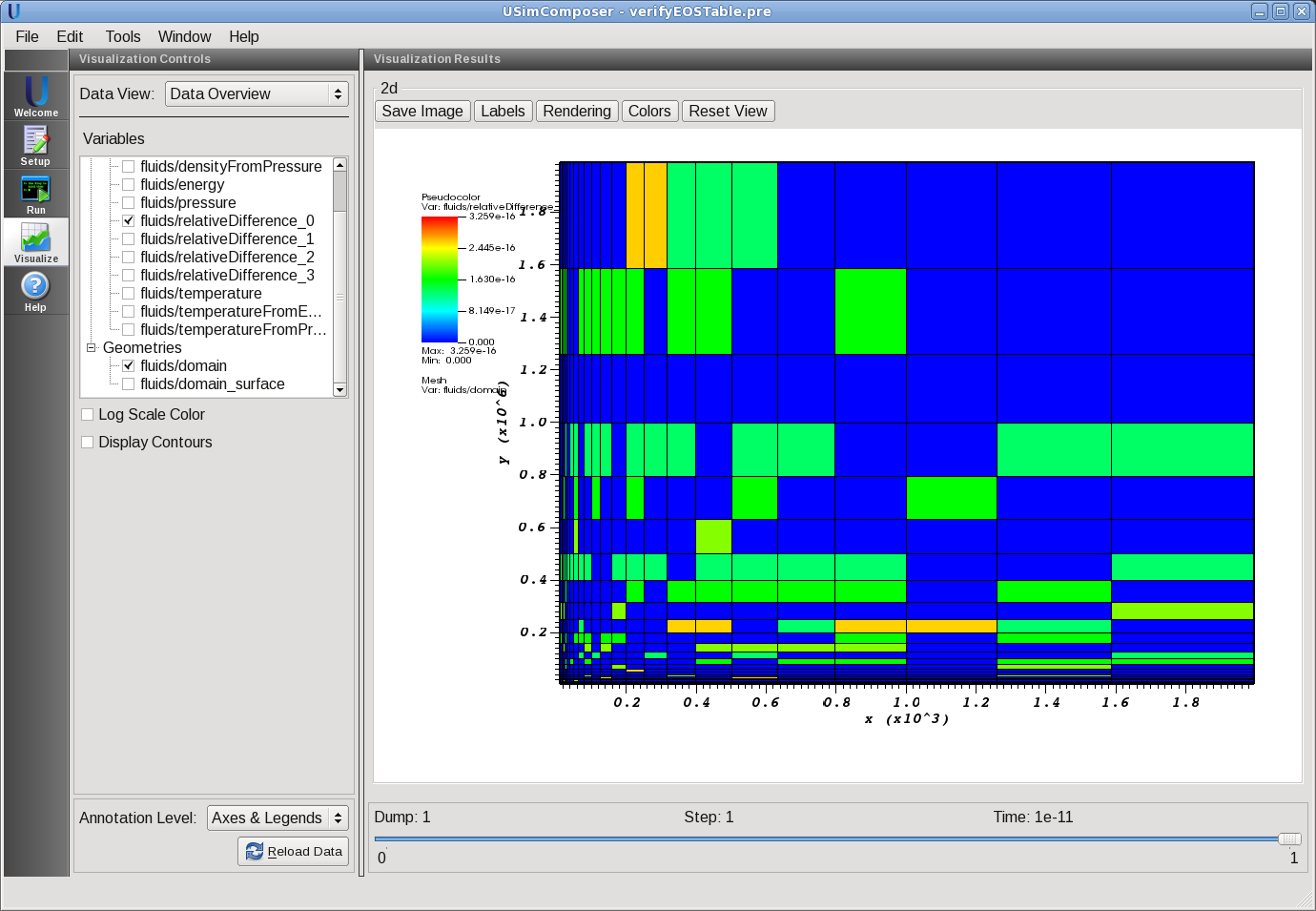
In this example, a logarithmic grid is configured that provides the initial values for temperature and density. The energy and pressure tables are evaluated and subsequently inverse operations are applied to recompute the density and temperature. There are four inverse operations, two for each of the energy and pressure tables. The relative difference of the inverse and initial densities and temperature are computed and should be accurate to machine precision in regions of interest.

This test can be performed with a USimHEDP license.

Creating the run space¶

The verify EOS Table example is accessed from within USimComposer by the following actions:

• Select the New from Template menu item in the File menu.
• In the resulting New from Template dialog, expand USimHEDP: High Energy Density Plasmas.
• Select Verify EOS Table and press the Choose button.
• In the Choose a name for the new runspace dialog, press the Save button to create a copy of this example in your run area.
• Press the Save And Process Setup button in the upper right corner of the Editor pane.

The basic example variables are editable in the Editor pane of the Setup window. After any change is made, the Save and Process Setup button must be pressed again before a new run commences.

Input file features¶

The following parameters can be varied to verify different EOS tables:

• TMIN - minimum temperature to check
• TMAX - maximum temperature to check
• NMIN - minimum mass density to check
• NMAX - maximum mass density to check
• EOSFILE - EOS table file name
• MATID - Material ID - required for SESAME only
• SPECIESMASS - Species mass - required for PROPACEOS only
• INPUTFORMAT - Input format - SESAME=0, PROPACEOS=1

Running the simulation¶

After performing the above actions, continue as follows:

• Proceed to the Run window as instructed by pressing the Run icon in the workflow panel.
• To run the simulation, click on the Run button in the upper right corner of the Logs and Output Files pane.

You will also see the engine log output in the Logs and Output Files pane. The run has completed when you see the output, “Engine completed successfully.”

Visualizing the results¶

After performing the above actions, continue as follows:

• Proceed to the Visualize window as instructed by pressing the Visualize icon in the workflow panel.
• Press the Open button to begin visualizing.
• Expand Scalar Data and click the check box for fluids/relativeDifference_0 to visualize the relative difference between the initial density and density computed from the inverse of the pressure EOS table as shown in Fig. 91.
• Check the other fluids/relativeDifference_X quantities 1-3 which correspond to the density from the inverse of the energy EOS table and the temperature from the inverse of the pressure and energy EOS tables, respectively.

The description of output parameters follows:

• density - initial density
• temperature - initial temperature
• energy - Energy computed from interpolation of the EOS table
• pressure - Pressure computed from interpolation of the EOS table
• densityFromPressure - Density computed through inverse interpolation of the EOS pressure table
• densityFromEnergy - Density computed through inverse interpolation of the EOS energy table
• temperatureFromPressure - Temperature computed through inverse interpolation of the EOS pressure table
• temperatureFromEnergy - Temperature computed through inverse interpolation of the EOS energy table
• relativeDifference - Quantities correspond to the relative difference of the initial and density from the inverse of the pressure and energy EOS tables and the temperature from the inverse of the pressure and energy EOS tables, respectively.

Figure 91: Visualization of the relative difference between the initial density and density computed from the inverse of the pressure EOS table.

Further experiments¶

• Change the material ID to check different materials
• Change the input file name to check different files
• When tables are not monotonic functions of density and temperature, note that incorrect results are expected. Ensure that the region of interest for computation produces valid results for the respective inverse operations that are used.