Shock Tube (shockTube.pre)¶

Problem description¶

This example computes shock tube problems for both hydrodynamic and magnetized flows. In essence, a shock tube is a 1D Riemann problem driven by discontinuous left and right states. Here, we provide a range of specific shock tubes for an ideal gas, including examples due to Einfeldt, Sod, Liska & Wendroff, Brio & Wu and Ryu & Jones. Further details, including reference solutions can be found in Stone et al. The Astrophysical Journal Supplement Series, Volume 178, Issue 1, article id. 137-177, pp. (2008).

This simulation can be performed with a USimBase license.

Creating the run space¶

The Shock Tube example is accessed from within USimComposer by the following actions:

• Select the New from Template menu item in the File menu.
• In the resulting New from Template dialog, expand USimBase: Basic Physics Capabilities.
• Select Shock Tube and press the Choose button.
• In the Choose a name for the new runspace dialog, press the Save button to create a copy of this example in your run area.
• Press the Save And Process Setup button in the upper right corner of the Editor pane.

The basic example variables are editable in the Editor pane of the Setup window as described below. After any change is made, the Save and Process Setup button must be pressed again before a new run may commence.

Input file features¶

The input file allows the user to set a variety of problem parameters related to the physics, initial conditions, domain and solver used for solving a shock tube problem.

The following parameters control the initial conditions of the shock tube:

• SHOCK_TUBE = EINFELDT1125, EINFELDT1203, SOD, SODLEVEQUE, SODTORO, LISKAWENDROFF, SLOW, BRIOWU, RYUJONES1a, RYUJONES1b, RYUJONES2a, RYUJONES2b, RYUJONES3a, RYUJONES3b, RYUJONES4a, RYUJONES4b, RYUJONES4c, RYUJONES4d selects the initial condition to run.
• REFERENCE_PRESSURE Pressure to scale the solution by in order to set the global sound speed.
• REFERENCE_DENSITY Density to scale the solution by in order to set the global sound speed.
• GAS_GAMMA Adiabatic index, or ratio of specific heats
• MU0 Vacuum permeability

The following parameters control the dimensionality, domain size and resolution of the simulation:

• NDIM = 1,2,3 selects whether to run the problem in one-, two- or three-dimensions.
• PAR_LENGTH sets the size of the domain in the direction parallel to the shock.
• PERP_LENGTH sets the size of the domain in the direction perpendicular to the shock.
• PAR_ZONES sets the number of zones in the direction parallel to the shock.
• PERP_ZONES sets the number of zones in the direction perpendicular to the shock.

The following parameters the length of the simulation and data output:

• TEND sets the end time for the simulation.
• NUMDUMPS sets the number of data dumps during the simulation
• WRITE_RESTART = False,True tells USim to output data necessary to restart the simulation. If this parameter is set to False then the Restart at Dump Number functionality in the Standard tab under Runtime Options in the Run window will not be available.

The following parameters control the USim solvers used to evolve the Kelvin-Helmholtz instability:

• TIME_ORDER = first,second,third,fourth sets the order of accuracy for the time-integration.
• DIFFUSIVE = False,True sets whether to use diffusive (but robust!) spatial integration schemes.
• DEBUG = False,True sets whether to output data for debugging a run. Warning: this will output A LOT of information!

Running the simulation¶

After performing the above actions, continue as follows:

• Proceed to the Run window as instructed by pressing the Run icon in the workflow panel.
• To run the simulation, click on the Run button in the upper right corner of the Logs and Output Files pane.

You will also see the engine log output in the Logs and Output Files pane. The run has completed when you see the output, “Engine completed successfully.”

Visualizing the results¶

After performing the above actions, continue as follows:

• Proceed to the Visualize window as instructed by pressing the Visualize icon in the workflow panel.
• Press the Open button to begin visualizing.
• Navigate to the “1-D Fields” Data View
• The visualization opens with four panels consisting of 1D line plots. The quantities are ‘fluids/density’ (mass density), ‘fluids/pressure’ (thermal pressure), ‘fluids/velocity_0’, ‘fluids/velocity_1’, ‘fluids/velocity_2’ (three components of the fluid velocity)
• Drag the slider at the bottom of the Visualization Results pane to Dump 10 to see results at the end of the simulation, as shown in Fig. 79.

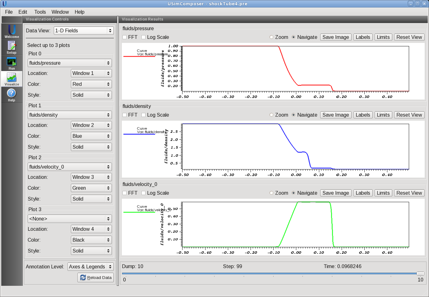
Figure 79: Visualization of gas pressure, fluid density and first component of the velocity for the default Shock Tube example.

Further experiments¶

• Change the adiabatic index of the gas (GAS_GAMMA) to see the effect of the gas having an different equation of state.
• Change the number of times a sound wave crosses the box (WAVE_CROSSINGS) to see the discontinuities propagate through the volume.
• Change the initial condition (SHOCK_TUBE) to the classic magnetized Brio & Wu shock tube (SHOCK_TUBE = BRIOWU).

Drag the slider at the bottom of the Visualization Results pane to Dump 10 to see results at the end of the simulation, as shown in Fig. 80.

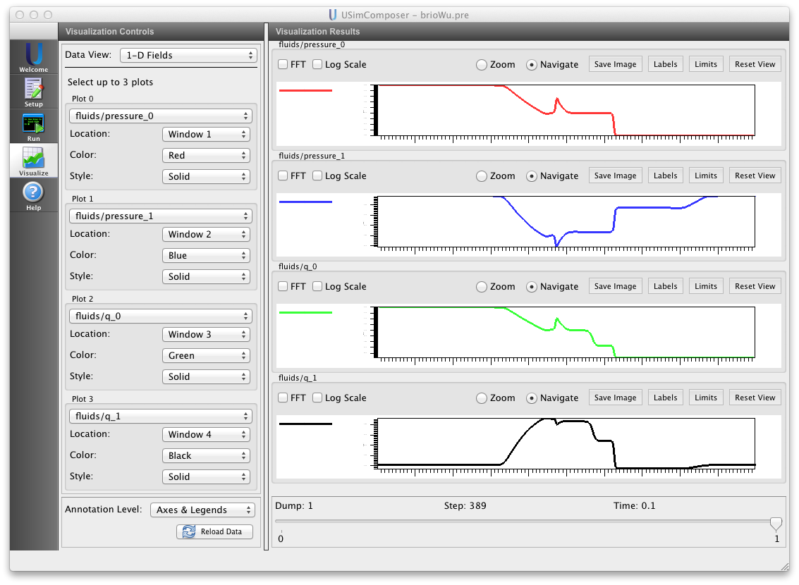
Figure 80: Visualization of gas pressure, fluid density and velocity for the default Brio & Wu shock tube.