Two-Fluid Magnetic Reconnection (gemChallenge.pre)¶

Problem description¶

This problem shows fast magnetic reconnection based on initial conditions from the GEM challenge magnetic reconnection problem. The model used is fully electromagnetic, two-fluid with semi-implicit time stepping to step over the plasma and cyclotron frequency. This approach shows significant speedup for problems where the cyclotron or plasma frequency dominates the time step.

Creating the run space¶

The Two-Fluid Magnetic Reconnection example is accessed from within USimComposer by the following actions:

• Select the New from Template menu item in the File menu.
• In the resulting New from Template dialog, expand USimHEDP: High Energy Density Plasmas.
• Select Two-Fluid Magnetic Reconnection and press the Choose button.
• In the Choose a name for the new runspace dialog, press the Save button to create a copy of this example in your run area.
• Press the Save And Process Setup button in the upper right corner of the Editor pane.

The basic example variables are editable in the Editor pane of the Setup window. After any change is made, the Save and Process Setup button must be pressed again before a new run commences.

Input file features¶

In the standard GEM challenge problem the initial conditions are set up in non-dimensional form. In this case we mimic this scenario by setting coefficients such as ion charge and permeability to 1.0 and then ensure that the ion thermal velocity is approximately 0.01c. A realistic electron to proton mass ratio is maintained. Divergence cleaning for the magnetic field is performed using the hyperbolic approach and Poisson equation is preserved using electric field diffusion.

In this simulation reconnected magnetic flux is stored using a dynVector. The reconnected flux is then one-half the integral of the absolute value of By along y=0. This reconnected flux can be compared with published results, though it will typically only converge to those results at high resolution. If possible, increase the resolution and run the simulation in parallel.

The key variables of the input file are exposed in the “Setup” window. These variables allow one to set the following fields

• CFL - CFL condition for the simulation
• TEND - Simulation end time (seconds).
• NUMDUMPS - Number of data dumps during the simulation
• SPECIES_CHARGE - Charge of the positive species.
• ION_MASS - Mass of the ion.
• ELECTRON_MASS - Mass of the electron.
• GAS_GAMMA - Specific heat ratio of the electron and ion fluid
• N0 - The peak ion number density
• LAMBDA - The current layer thicknesss
• B0 - The X magnetic field at infinity
• PERTURBATION_FACTOR - The factor that B0 is multiplied by to define the size of the perturbation
• SPEED_OF_LIGHT - Speed of light
• EPSILON0 - Permeability of free space
• BP - Magnetic correction potential field divergence correction speed factor. The correction speed is given by speed=BP*c so the value BP should be near 1.0 .
• FLUID_NUMERICAL_FLUX - specifies the Riemann solver used to calculate an upwind approximation to the flux tensor. For hydrodynamic problems, options include localLaxFlux, hlleFlux, hllcEulerFlux. For magnetohydrodynamic problems, options include localLaxFlux, hlleFlux, hlldMhdFlux, fWaveFlux. For more general systems, options include localLaxFlux, hlleFlux, fWaveFlux.
• EM_NUMERICAL_FLUX - specifies the Riemann solver used to calculate an upwind approximation to the flux tensor. For hydrodynamic problems, options include localLaxFlux, hlleFlux, hllcEulerFlux. For magnetohydrodynamic problems, options include localLaxFlux, hlleFlux, hlldMhdFlux, fWaveFlux. For more general systems, options include localLaxFlux, hlleFlux, fWaveFlux.
• TIME_ORDER=first,second,third,fourth - sets the order of accuracy for the time-integration.
• LIMITER=muscl,minmod,none - specifices the spatial limiting method used in reconstructing primary variables to use to ensure that method remains total value diminishing (TVD).
• NX - Number of cells in the x direction
• NY - Number of cells in the y direction
• NZ - Number of cells in the z direction (3D only)
• X_MIN - lower X position of grid
• X_MAX - upper X position of grid
• Y_MIN - lower Y position of grid
• Y_MAX - upper Y position of grid
• Z_MIN - lower Z position of grid (only in 3D)
• Z_MAX - upper Z position of grid (only in 3D)

Running the simulation¶

After performing the above actions, continue as follows:

• Proceed to the Run window as instructed by pressing the Run icon in the workflow panel.
• To run the simulation, click on the Run button in the upper right corner of the Logs and Output Files pane.

You will also see the engine log output in the Logs and Output Files pane. The run has completed when you see the output, “Engine completed successfully.”

Visualizing the results¶

After performing the above actions, continue as follows:

• Proceed to the Visualize window as instructed by pressing the Visualize icon in the workflow panel.
• Press the Open button to begin visualizing.
• In the Data View dropdown menu, select History. The history field will provide you with access to dynVectors, in this case the reconnected flux. Plot 0 selects integratedFlux. The image below shows the result of a complete simulation Fig. 87.

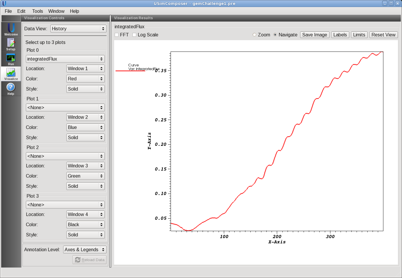
Figure 87: Visualization of the integratedFlux history in the Two-Fluid Magnetic Reconnection example

Further experiments¶

• Decreasing the plasma layer thickness (LAMBDA) increases the initial reconnection rate.
• Decreasing the SPECIES_CHARGE reduces the magnetization (by increasing the Larmor radius of the electrons and ions) and prevents the magnetic field from maintaining equilibrium. Increasing the SPECIES_CHARGE does the opposite, the field is tied more closely to the plasma. Fast reconnection can occur in this case. However, it likely requires much higher resolution to effectively resolve the reconnection layer.