Blunt-Body Reentry Vehicle (ramC.pre)¶

Problem description¶

Reentry of RAMC-type module is simulated. The aerothermal heating due the formation of shock wave and the resulting weakly ionized plasma are simulated at an altitude of 61 km. Navier-Stokes equations are used for flow simulation. Thermophysical properties of air are computed internally using kinetic theory. This simulation is carried out for zero angle of attack and hence axi-symmetric form of equations are used. 7 species air chemistry model is used to obtain the species densities. Given distribution of temperature along with mass injection can be specified on the surface. Na, Ca, and K are injected. Ca and Na are injected in the nose cap region. K and Na are injected from the lateral surface. This simulation considers 10 species in total.

This simulation can be performed with USimHS license.

Creating the run space¶

The ramC example is accessed from within USimComposer by the following actions:

• Select the New from Template menu item in the File menu.
• In the resulting New from Template dialog, expand USimHS: Hypersonics.
• Select ramC and press the Choose button.
• In the Choose a name for the new runspace dialog, press the Save button to create a copy of this example in your run area.
• Press the Save And Process Setup button in the upper right corner of the Editor pane.

The basic example variables are editable in the Editor pane of the Setup window. After any change is made, the Save and Process Setup button must be pressed again before a new run commences.

Input file features¶

The input folder has externally generate mesh file using Cubit. The following parameters can be varied to simulate different flow regimes.

• TSTART - Simulation start time (seconds).
• TEND - Simulation end time (seconds).
• NUMDUMPS - Number of data dumps during the simulation
• GRIDFILE - name of grid file
• REACTIONS_ATOMIC_DATA - name of the file containing reactions and atomic data
• W0 - z-component of free stream velocity
• FREESTREAM_DENSITY - free stream density
• FREESTREAM_TEMPERATURE - free stream temperature
• SURFACE_TEMPERATURE - surface temperature
• INJECTION_DENSITY1 - density at injection boundary1
• INJECTION_VELOCITY1 - X component velocity at injection boundary1
• MWinj1_1 - molecular weight of species 1
• MWinj1_2 - molecular weight of species 2
• MFinj1_1 - mass fraction of species 1
• MFinj1_2 - mass fraction of species 2
• INJECTION_DENSITY2 - density at injection boundary2
• INJECTION_VELOCITY2 - X component velocity at injection boundary2
• MWinj2_1 - molecular weight of species 1
• MWinj2_2 - molecular weight of species 2
• MFinj2_1 - mass fraction of species 1
• MFinj2_2 - mass fraction of species 2
• NUMERICAL_FLUX - specifies the Riemann solver used to calculate an upwind approximation to the flux tensor. For hydrodynamic problems, options include localLaxFlux, hlleFlux, hllcEulerFlux. For magnetohydrodynamic problems, options include localLaxFlux, hlleFlux, hlldMhdFlux, fWaveFlux. For more general systems, options include localLaxFlux, hlleFlux, fWaveFlux.
• TIME_ORDER=first,second,third,fourth - sets the order of accuracy for the time-integration.
• CFL_CONVECTIVE - CFL condition number for convective terms
• VISCOUS_DIFF_TIMESTEP_FACTOR - Factor to further decrease the internally computed time step based on kinematic viscosity
• THERMAL_DIFF_TIMESTEP_FACTOR - Factor to further decrease the internally computed time step based on thermal diffusicity
• BASEMENT_TEMPERATURE - least possible temperature in the domain (K).

Running the simulation¶

After performing the above actions, continue as follows:

• Proceed to the Run window as instructed by pressing the Run icon in the workflow panel.
• To run the simulation, click on the Run button in the upper right corner of the Logs and Output Files pane.

You will also see the engine log output in the Logs and Output Files pane. The run has completed when you see the output, “Engine completed successfully.”

Visualizing the results¶

After performing the above actions, continue as follows:

• Proceed to the Visualize window as instructed by pressing the Visualize icon in the workflow panel.
• Press the Open button to begin visualizing.
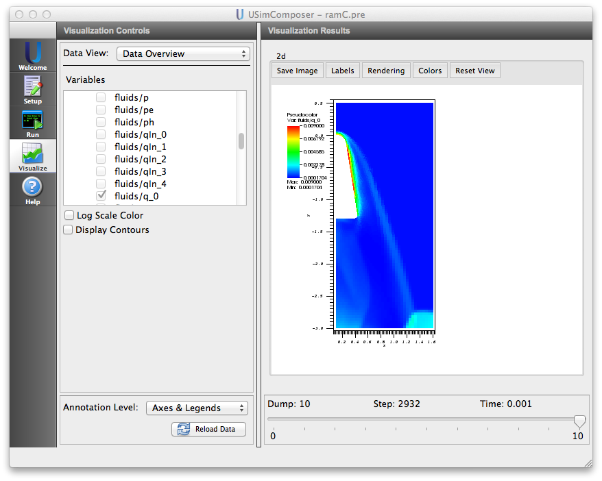
• Expand Scalar Data and click the check box for fluids/q_0 to visualize the density distribution.
• Drag the slider at the bottom of the Visualization Results pane to move through the simulation in time. The fluid density distribution at the end of the simulation is shown in Fig. 97.

The following parameters can also be visualized:

• a speed of sound
• mwAvg average molecular weight of gas mixture (molecular weight varies due to the change in composition of gas)
• cpR_0 - cpR_9 constant pressure specific heat of species
• cpAvg average specific heat of fluid
• gammaAvg specific heat ratio of fluid
• p total pressure
• pe electron pressure
• ph heavy particle pressure
• q_0 mass density
• q_1,q_2,q_3 momentum components
• q_4 energy density
• speciesDens_0 - speciesDens_9 number densities of the species
• temperature average temperature of the mixture
• velocity_0,velocity_1,velocity_2 three components of velocity

Species indices are 0 to 6 (N2,N,O2,O,NO,NO+,e,Ca,Na,K).

Figure 97: Visualization of density distribution for the Blunt-Body Reentry Vehicle example.

Further experiments¶

• The freestream velocity W0 may be changed to simulate different Mach numbers at a given altitude. Increase in electron density as a result of increased aerothermal heating can be noticed.
• The freestream temperature and density can be changed to simulate the changes in altitude. Lets say at 50 km altitude, the density and temperature of air are 0.000978 \(kg/m^3\) and 270 K. Simulation without changing the freestream air speed shows that the electron density increases mainly due to the increase in freestream density.
• Change the surface temperature, mass injection densities and velocities. The injection species may also be changed by changing their atomic properties both in the input file and air7SpeciesAb.txt file.