Solving Problems on Advanced Structured Meshes in USim
In Using USim to solve the Euler Equations we discussed the basic methods used by USim to solve the Euler equations. Next, in Using USim to solve the Magnetohydrodynamic Equations, we extended these ideas to solve the MHD equations in one-dimension and showed how USimBase simulations for both the Euler and MHD equations follow the same basic pattern. Then, in Solving Multi-Dimensional Problems in USim, we built on these concepts to demonstrate how to use USim to solve the Euler and MHD equations in multi-dimensions, how to utilize more advanced boundary conditions and how to apply external forces (such as gravity) to the equations. In this tutorial, we extend these ideas to demonstrate how USim can solve problems in axisymmetric curvilinear coordinates and how to use two- and three-dimensional body fitted meshes to solve problems around simple geometries.
Contents
Solving Problems in Axi-Symmetric Curvilinear Coordinates
An example of using USim to solve the MHD equations in axi-symmetric curvilinear coordinates is found in Unstable Plasma zPinch (zPinch.pre).
Adding a Simulation Grid
The use of axisymmetric cylindrical coordinates in this problem is specified through the use of the grid:
addCylindricalGrid(lowerBounds, upperBounds, numCells, periodicDirections)
This macro is documented at Grid Macro and follows the same pattern that we have seen previously for logically structured Cartesian grids:
lowerBounds:- Vector of coordinates for lower edge of grid, lowerBounds = [ RMIN ZMIN PHIMIN ]
upperBounds:- Vector of coordinates for upper edge of grid, upperBounds = [ RMAX ZMAX PHIMAX ]
numCells:- Vector of number of cells in grid, numCells = [ NR NZ NPHI ]
periodicDirections:List of directions that are periodic
periodicDirections = [ 0 ] (R-direction periodic)
periodicDirections = [ 0 1 ] (R,Z-directions periodic)
periodicDirections = [ 0 1 2 ] (R,Z,PHI-directions periodic)
Using the addCylindricalGrid macro automatically tells the rest of the USim solvers to use the cylindrical form of the operator. If a cylindrical form of an operator is not available, USim will stop with an error message.
Note
Cylindrical grids in USim are designed with axisymmetric coordinates in mind, so a one-dimensional mesh simulates the \(R\) coordinate, a two-dimensional mesh simulates the \((R,Z)\) coordinates and a three-dimensional mesh simulates the \((R,Z,\phi)\) coordinates.
Creating a Fluid Simulation
The initial conditions for the Unstable Plasma zPinch (zPinch.pre) in axisymmetric cylindrical coordinates are given by:
Step 1:
addVariable(gas_gamma,GAS_GAMMA)
addVariable(mu0,MU0)
addVariable(invSqrtMu0,INV_SQRT_MU0)
addVariable(Rp,RP)
addVariable(n_0,N0)
addVariable(j_0,J0)
addVariable(p_0,P0)
addVariable(mi,MI)
addVariable(k,WAVENUMBER)
addVariable(alpha,BASE_PRESSURE_RATIO)
addVariable(perturb,PERTURBATION_AMPLITUDE)
Step2:
addPreExpression(r = x)
addPreExpression(Z = y)
addPreExpression(phi = z)
addPreExpression(rho = if(r<Rp, mi*n_0*(alpha+(1.0-(r*r)/(Rp*Rp))), mi*n_0*alpha))
addPreExpression(vr = 0.0)
addPreExpression(vphi = 0.0)
addPreExpression(vz = 0.0)
addPreExpression(pr = if(r < Rp, p_0-0.25*mu0*j_0*j_0*r*r, alpha*0.25*mu0*j_0*j_0*Rp*Rp))
addPreExpression(br = 0.0)
addPreExpression(bphi = if(r < Rp, -0.5*r*mu0*j_0*(1.0+perturb*sin(k*Z)), -0.5*(Rp*Rp/r)*mu0*j_0*(1.0+perturb*sin(k*Z))))
addPreExpression(bz = 0.0)
addPreExpression(psi = 0.0)
Step 3:
addExpression(rho)
addExpression(rho*vr)
addExpression(rho*vphi)
addExpression(rho*vz)
addExpression(pr/(gas_gamma-1.0) + 0.5*rho*(vr*vr+vphi*vphi+vz*vz)+0.5*((br*br+bphi*bphi+bz*bz)/mu0))
addExpression(br*invSqrtMu0)
addExpression(bphi*invSqrtMu0)
addExpression(bz*invSqrtMu0)
addExpression(psi)
Note
While the ordering of coordinates on cylindrical grids in USim is \((R,Z,\phi)\), the components of vectors (such as the momentum and magnetic field defined in step 3 above) take the order \((\hat{\mathbf{R}},\hat{\mathbf{\phi}},\hat{\mathbf{Z}})\). Many issues in simulations involving cylindrical coordinates originate in an incorrect ordering of vector components.
Putting it all Together
We can then extend the underlying pattern for USimBase simulations to incorporate curvilinear coordinates:
# Are we solving the MHD equations?
$ MHD = True

# Are we using cylindrical coordinates?
$ CYLINDRICAL = True

# Import macros to setup simulation
$ import fluidsBase.mac
# if MHD
$ import idealmhd.mac
$ else
$ import euler.mac
$ endif

# Specify parameters for the specific physics problem
$ PARAM_1 = <value>
$ PARAM_2 = <value>
$ PARAM_N = <value>

# Initialize a USim simulation
$ if MHD
initializeFluidSimulation(NDIM,0.0,END_TIME,NUMDUMPS,CFL,GAS_GAMMA,MU0,WRITE_RESTART,DEBUG)
$ else
initializeFluidSimulation(NDIM,0.0,END_TIME,NUMDUMPS,CFL,GAS_GAMMA,WRITE_RESTART,DEBUG)
$ endif

# Setup the grid
$ if CYLINDRICAL
addCylindricalGrid(lowerBounds, upperBounds, numCells, periodicDirections)
$ else
addGrid(lowerBounds, upperBounds, numCells, periodicDirections)
$ endif

# Create data structures needed for the simulation
createFluidSimulation()

# Specify initial condition
# Step 1: Add Variables
addVariable(NAME,<value>)

# Step 2: Add Pre-Expressions
addPreExpression(<PreExpression>)

# Step 3: a) Add expressions specifying initial condition on density,
# momentum
addExpression(<expression>)
$ if MHD
# Step 3: b) Add expression specifying initial conditions on total
# energy, magnetic field, correction potential
addExpression(<expression>)
$ else
# Step 3: b) Add expression specifying initial conditions on total
# energy
addExpression(<expression>)
$ endif

# Add the spatial discretization of the fluxes
finiteVolumeScheme(DIFFUSIVE)

# Boundary conditions
boundaryCondition(<boundaryCondition,entity>)

# Time integration
timeAdvance(TIME_ORDER)

# Run the simulation!
runFluidSimulation()
An Example Simulation
The input file for Unstable Plasma zPinch (zPinch.pre) in the USimBase package demonstrates each of the concepts described above to evolve the z-Pinch problem in two-dimensional magnetohydrodynamics. Executing this input file within USimComposer and switching to the Visualize tab yields the plots shown in Fig. 4.
Note
For more depth, you can view the actual input blocks to Ulixes in the Setup window by choosing Save And Process Setup and then clicking on the zPinch.in file. In the .in file all macros are expanded to produce input blocks.
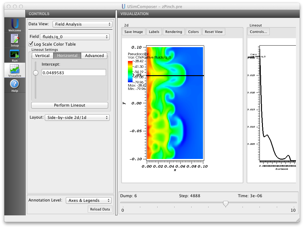
Figure 4: Visualization tab in USimComposer after executing the Unstable plasma z-Pinch input file for the tutorial.
Solving Problems on Two-Dimensional Body-Fitted Meshes in USim
This tutorial is based on the Magnetized Ramp Flow (rampFlow.pre) example in USimBase, which we use to demonstrate the creation of two-dimensional body fitted meshes.
Adding a Simulation Grid
The Ramp Flow simulation uses a bodyFitted (1d, 2d, 3d) grid, which is added to the simulation through the addBodyFittedGrid macro:
addBodyFittedGrid(lowerBounds, upperBounds, numCells, periodicDirections)
The options for this macro are documented in Grid Macro. For completeness, we include them here:
lowerBounds:- Vector of coordinates for lower edge of grid, lowerBounds = [ XMIN YMIN ZMIN ]
upperBounds:- Vector of coordinates for upper edge of grid, upperBounds = [ XMAX YMAX ZMAX ]
numCells:- Vector of number of cells in grid, numCells = [ NX NY NZ ]
periodicDirections:List of directions that are periodic
periodicDirections = [ 0 ] (x-direction periodic)
periodicDirections = [ 0 1 ] (x,y-directions periodic)
periodicDirections = [ 0 1 2 ] (x,y,z-directions periodic)
Now that the body-fitted grid has been created, it is possible to transform the coordinates of the grid into the desired shaped. This is a three-step process, much like specifying an initial condition:
- Use addGridVariable to add variables that are independent of grid position.
- Use addGridPreExpression to add quantities that are functions of grid position, variables and any previously defined PreExpression in this block. Evaluated before expressions and the result is not accessible outside of this block. Any number of PreExpressions can be added.
- Use addGridExpression to define the new coordinates in the grid. The order of the expressions correspond to the order of the coordinates in the grid and there must be the same number of expressions as dimensions in the grid.
For the RampFlow example, the GridVariables added in Step 1 in the above process are:
# Grid properties
addGridVariable(xmin,XIN)
addGridVariable(xmax,XUP)
addGridVariable(ymax,YUP)
addGridVariable(slope,$math.tan(math.pi*THETA/180)$)

# Numbers of cells
addGridVariable(inletCells,1.0*NXI)
addGridVariable(rampCells,1.0*NXR)
addGridVariable(yCells,$1.0*NY$)

# x direction cell spacing in computational space
addGridVariable(dxc,$1.0/(NXI+NXR)$)
# y direction cell spacing in computational space
addGridVariable(dyc,$1.0/NY$)
# z direction cell spacing in computational space
Next, the GridPreExpressions added in Step 2 in the above process are:
# Grid preExpressions
addGridPreExpression(ix=rint(x/dxc))
addGridPreExpression(iy=rint(y/dyc))
addGridPreExpression(dxi=xmin/inletCells)
addGridPreExpression(dxr=(xmax-xmin)/rampCells)
addGridPreExpression(xp=if(inletCells>=ix,dxi*ix,xmin+dxr*(ix-inletCells)))
addGridPreExpression(dyi = ymax/yCells)
addGridPreExpression(b = -slope*xmin)
addGridPreExpression(y0 = slope*xp + b)
addGridPreExpression(dyr = (ymax-y0)/yCells)
addGridPreExpression(yp=if(inletCells>=ix,dyi*iy,y0+dyr*iy))
Finally, the GridExpressions added in Step 3 in the above process are:
addGridExpression(xp)
addGridExpression(yp)
The bodyFitted Grid in USim is an extension of the cart grid. The cart Grid lays out the grid in a uniform manner and provides an x-y coordinate for each of the vertices of the cells. The bodyFitted grid allows the user to modify the locations of these x-y vertices. The lowerBounds upperBounds and numCells parameters set up the uniform cartesian grid and its vertices. The vertices of this cartesian grid are then modified according to the GridExpressions which defines the mapping from the cartesian grid to the bodyFitted grid, therefore if we specify:
addGridExpression(x*x)
addGridExpression(y*y)
then the cartesian grid is mapped to a grid with where x and y vary quadratically. USim loops through every vertex and replaces the cartesian vertex with the new vertex specified by each of the addGridExpression macros. The user must be careful to make sure that the new vertices are a result of simple stretching the cartesian grid so that cells in the body fitted grid do not overlap.
Note
In the body fitted grid, ghost cells are also mapped using the addGridExpression macros. Ghost cells add an extra layer to the grid beyond what is specified by cells. The location of these additional vertices can be computed by adding additional cells to the cartesian grid. In many cases it is also important that the mapping of these ghost cells do not produce overlapping cells which can result in negative areas and misdirected tangents and normals.
An Example Simulation
The input file for the problem Ramp Flow in the USimBase package demonstrates each of the concepts described above. Executing this input file within USimComposer and switching to the Visualize tab yields the plots shown in Fig. 5.
Note
For more depth, you can view the actual input blocks to Ulixes in the Setup window by choosing Save And Process Setup and then clicking on the rampFlow.in file. In the .in file all macros are expanded to produce input blocks.
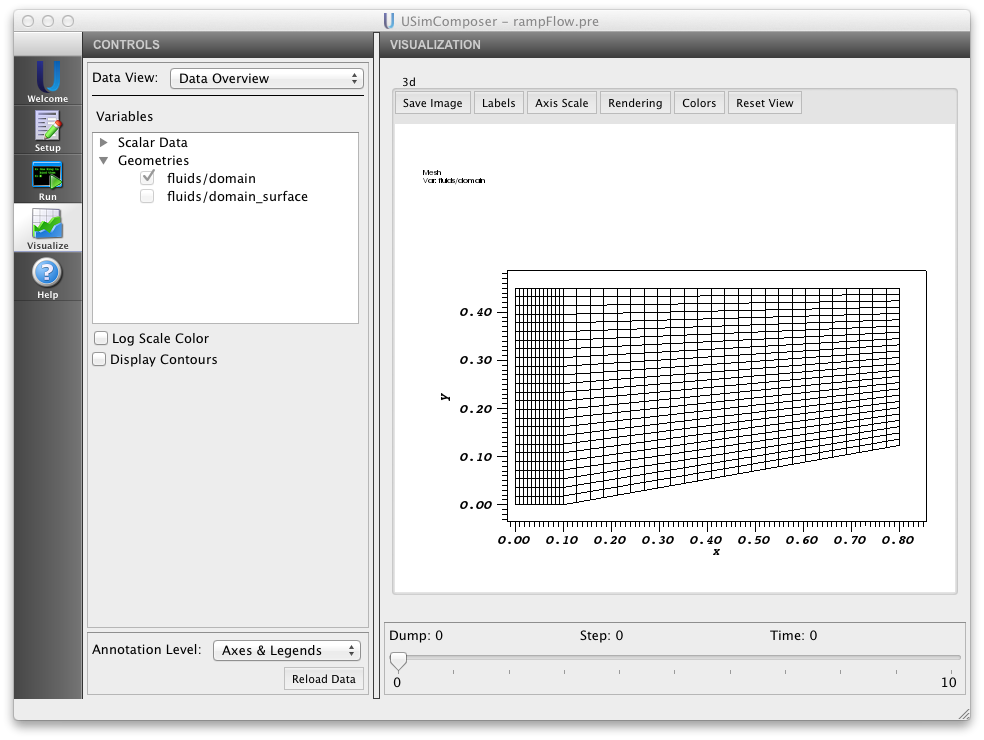
Figure 5: Visualization of mesh geometry in USimComposer after executing the MHD Ramp Flow input file for the tutorial.
Solving Problems on Three-Dimensional Body-Fitted Meshes in USim
The input file for Unstable Plasma zPinch (zPinch.pre) in the USimBase package demonstrates each of the concepts described above to evolve the z-Pinch problem in three-dimensional magnetohydrodynamics
Adding a Simulation Grid
The three-dimensional version of the zPinch simulation uses a bodyFitted (1d, 2d, 3d) grid, which is added to the simulation through the addBodyFittedGrid macro:
addBodyFittedGrid(lowerBounds, upperBounds, numCells, periodicDirections)
The options for this macro are documented in Grid Macro. For completeness, we include them here:
lowerBounds:- Vector of coordinates for lower edge of grid, lowerBounds = [ XMIN YMIN ZMIN ]
upperBounds:- Vector of coordinates for upper edge of grid, upperBounds = [ XMAX YMAX ZMAX ]
numCells:- Vector of number of cells in grid, numCells = [ NX NY NZ ]
periodicDirections:List of directions that are periodic
periodicDirections = [ 0 ] (x-direction periodic)
periodicDirections = [ 0 1 ] (x,y-directions periodic)
periodicDirections = [ 0 1 2 ] (x,y,z-directions periodic)
In this example, we use the body-fitted grid to transform a three-dimensional cylindrical mesh into a three-dimensional \((X,Y,Z)\) mesh that utilizes a cylindrical distribution. To accomplish this, we only have to perform the third step of the three-step process above:
addGridExpression(x*cos(y))
addGridExpression(x*sin(y))
addGridExpression(z)
Creating a Fluid Simulation
In order to specify the initial condition on a three-dimensional Cartesian mesh when we start from a cylindrical initial condition, we need to transform components of vectors from cylindrical to cartesian coordinates. We can do this during the specification of the initial condition:
Step 1
addVariable(gas_gamma,GAS_GAMMA)
addVariable(mu0,MU0)
addVariable(invSqrtMu0,INV_SQRT_MU0)
addVariable(Rp,RP)
addVariable(n_0,N0)
addVariable(j_0,J0)
addVariable(p_0,P0)
addVariable(mi,MI)
addVariable(k,WAVENUMBER)
addVariable(alpha,BASE_PRESSURE_RATIO)
addVariable(perturb,PERTURBATION_AMPLITUDE)
Step 2
# Compute cylindrical coordinatees based on our x,y,z coordinates in
# the grid
addPreExpression(r = sqrt(x^2+y^2))
addPreExpression(phi = atan2(y,x))
addPreExpression(Z = z)

# Setup our plasma parameters in cylindrical coordinates
addPreExpression(rho = if(r<Rp, mi*n_0*(alpha+(1.0-(r*r)/(Rp*Rp))), mi*n_0*alpha))
addPreExpression(vr = 0.0)
addPreExpression(vphi = 0.0)
addPreExpression(vz = 0.0)
addPreExpression(pr = if(r < Rp, p_0-0.25*mu0*j_0*j_0*r*r, alpha*0.25*mu0*j_0*j_0*Rp*Rp))
addPreExpression(br = 0.0)
addPreExpression(bphi = if(r < Rp, -0.5*r*mu0*j_0*(1.0+perturb*sin(k*Z)), -0.5*(Rp*Rp/r)*mu0*j_0*(1.0+perturb*sin(k*Z))))
addPreExpression(bz = 0.0)
addPreExpression(psi = 0.0)

# Transform from cylindrical coordinates into Cartesian.
addPreExpression(vx = vr*cos(phi)+vphi*sin(phi))
addPreExpression(vy = vr*sin(phi)-vphi*cos(phi))
addPreExpression(bx = br*cos(phi)+bphi*sin(phi))
addPreExpression(by = br*sin(phi)-bphi*cos(phi))
Step 3
# Specify initial condition according to cartesian vector components
addExpression(rho)
addExpression(rho*vx)
addExpression(rho*vy)
addExpression(rho*vz)
addExpression(pr/(gas_gamma-1.0) + 0.5*rho*(vx*vx+vy*vy+vz*vz)+0.5*((bx*bx+by*by+bz*bz)/mu0))
addExpression(bx*invSqrtMu0)
addExpression(by*invSqrtMu0)
addExpression(bz*invSqrtMu0)
addExpression(psi)
An Example Simulation
The input file for Unstable Plasma zPinch (zPinch.pre) in the USimBase package with NDIM=3 demonstrates each of the concepts described above to evolve the z-Pinch problem in three-dimensional magnetohydrodynamics.
Note
For more depth, you can view the actual input blocks to Ulixes in the Setup window by choosing Save And Process Setup and then clicking on the zPinch.in file. In the .in file all macros are expanded to produce input blocks.