Multi-Fluids with Collisions (collisionalMultiFluid.pre)
Keywords:
-
Multi-Fluid Collisions
Problem description
This problem shows collisions between three (separate) fluid species in a simple shock problem and allows one to compare it with the single-fluid solution. In the highly collisional regime the multi-fluid problem converges to the single fluid case.
This simulation can be performed with a USimHEDP license.
Creating the run space
The Multi-Fluids with Collisions example is accessed from within USimComposer by the following actions:
- Select the New from Template menu item in the File menu.
- In the resulting New from Template dialog, expand USimHEDP: High Energy Density Plasmas.
- Select Multi-Fluids with Collisions and press the Choose button.
- In the Choose a name for the new runspace dialog, press the Save button to create a copy of this example in your run area.
- Press the Save And Process Setup button in the upper right corner of the Editor pane.
The basic example variables are editable in the Editor pane of the Setup window. After any change is made, the Save and Process Setup button must be pressed again before a new run commences.
Input file features
The following parameters can be varied to look at the effects of collisionality on the shock solution:
- NUMDUMPS - Number of data dumps during the simulation
- XUPPER - Domain size
- PRESSURE - Reference pressure of the gas
- DENSITY - Reference density of the gas
- GAMMA - Gas constant
- PRL - the total pressure on the left half of the domain.
- RHOL - the total density on the left half of the domain.
- PRR - the total pressure on the right half of the domain.
- RHOR - the total density on the right half of the domain.
- FRAC1L - the fraction of gas 1 on the left half initially.
- FRAC2L - the fraction of gas 2 on the left half initially.
- FRAC3L - the fraction of gas 3 on the left half initially.
- FRAC1R - the fraction of gas 1 on the right half initially.
- FRAC2R - the fraction of gas 2 on the right half initially.
- FRAC3R - the fraction of gas 3 on the right half initially.
- MI - Reference mass of ion
- DI - Reference diameter of ion
- MI1 - Mass of ion1
- MI2 - Mass of ion2
- MI3 - Mass of ion3
- DI1 - Diameter of ion1
- DI2 - Diameter of ion2
- DI3 - Diameter of ion3
Running the simulation
After performing the above actions, continue as follows:
- Proceed to the Run window as instructed by pressing the Run icon in the workflow panel.
- To run the simulation, click on the Run button in the upper right corner of the Logs and Output Files pane.
You will also see the engine log output in the Logs and Output Files pane. The run has completed when you see the output, “Engine completed successfully.”
Visualizing the results
After performing the above actions, continue as follows:
- Proceed to the Visualize window as instructed by pressing the Visualize icon in the workflow panel.
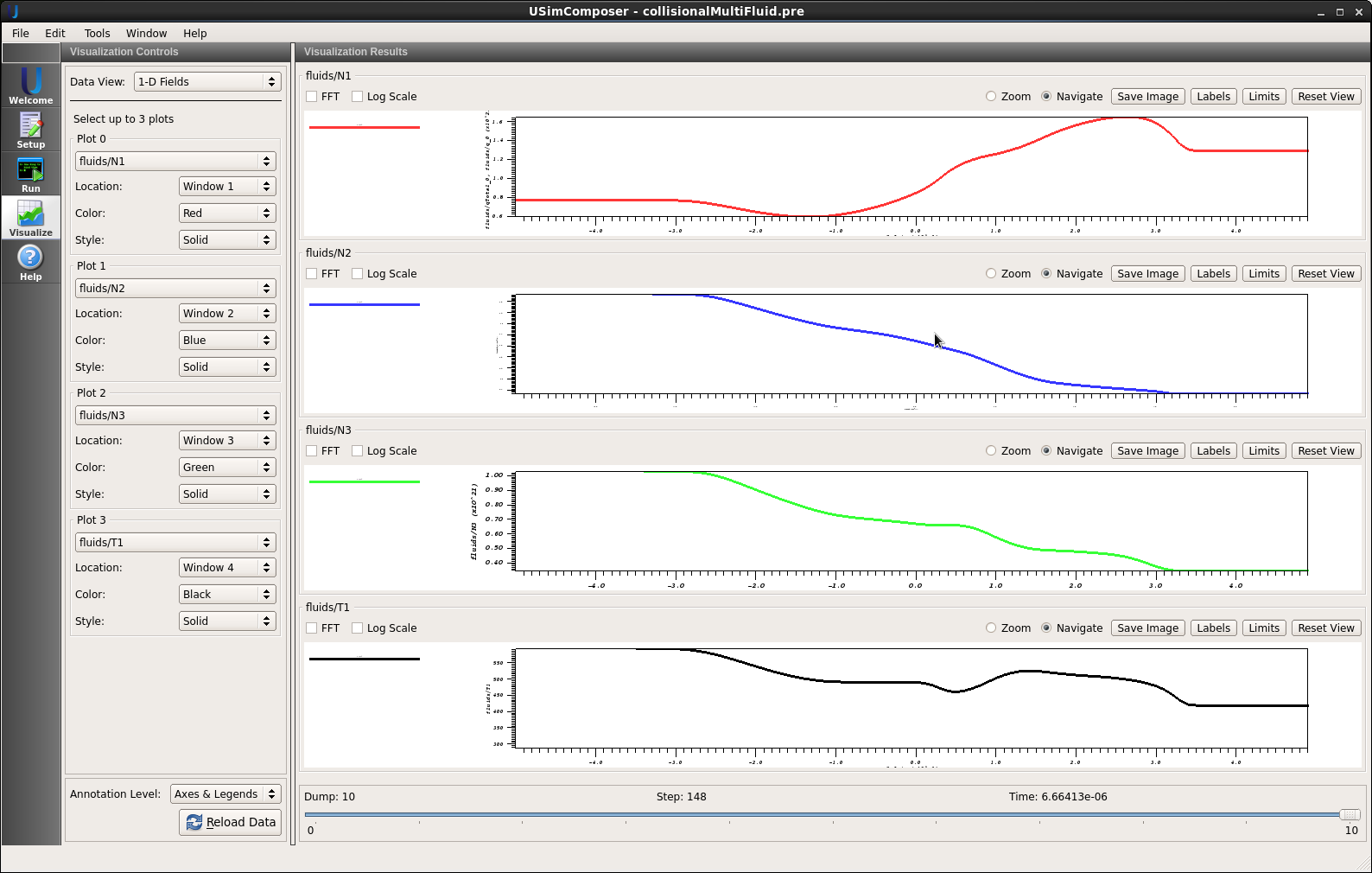
- Press the Open button to begin visualizing. The visualization opens with four panels consisting of 1D line plots.
- Drag the slider at the bottom of the Visualization Results pane to
see results at the end of the simulation, as shown in
Fig.
Fig. #collisionalmultifluidvizwin.
The following values can be visualized
- N1,N2,N3 the number densities for species 1, 2 and 3
- T1,T2,T3 the temperatures for species 1, 2 and 3
- V1_0,V1_1,V1_2 the velocity components for species 1
- V2_0,V2_1,V2_2 the velocity components for species 2
- V3_0,V3_1,V3_2 the velocity components for species 3
- collisionMatrix_0 through collisionMatrix_8 the collisional cross frequencies between species
- q1_0,q1_1,q1_2,q1_3,q1_4 the mass density, momentum density and energy of the first species
- q2_0,q2_1,q2_2,q2_3,q2_4 the mass density, momentum density and energy of the second species
- q3_0,q3_1,q3_2,q3_3,q3_4 the mass density, momentum density and energy of the third species
- qTotal_0,qTotal_1,qTotal_2,qTotal_3,qTotal_4 the mass density, momentum density and energy of the sum of the 3 species
Further experiments
- Increase RHOL and RHOR by a factor of 10 and the fluids will become much more collisional, producing the standard sod shock result.
