Dense Plasma Focus (densePlasmaFocus.pre)¶

Problem description¶

This problem solves a simple dense plasma focus (DPF) using a two-temperature MHD model with a user-specified equation of state on an unstructured grid in axisymmetric geometry. The dense plasma focus is a fusion concept envisioned as both a power source, neutron source, and even high-powered propulsion. The DPF is also similar to other plasma accelerators such as the magneto plasma dynamic (MPD) thruster, in which the plasma is accelerated by the self field created by the current running through the plasma.

Creating the run space¶

The Dense Plasma Focus example is accessed from within USimComposer by the following actions:

• Select the New from Template menu item in the File menu.
• In the resulting New from Template dialog, expand USimHEDP: High Energy Density Plasmas.
• Select Dense Plasma Focus and press the Choose button.
• In the Choose a name for the new runspace dialog, press the Save button to create a copy of this example in your run area.
• Press the Save And Process Setup button in the upper right corner of the Editor pane.

The basic example variables are editable in the Editor pane of the Setup window. After any change is made, the Save and Process Setup button must be pressed again before a new run commences.

Input file features¶

The input file allows the user to specify the number density of the plasma (N0), the temperature of the plasma (T), a constant resistivity (ETA), the atomic weight of the plasma species (ATOMIC_WEIGHT), and the current flowing through the plasma (CURRENT). In addition, many numerical parameters can be set through the input file.

The key variables of the input file are exposed in the “Setup” window. These variables allow one to set the following fields

• GRIDFILE - Name of the mesh file
• CFL - CFL condition for the simulation
• TEND - Simulation end time (seconds).
• NUMDUMPS - Number of data dumps during the simulation
• ATOMIC_WEIGHT - Atomic weight of ion
• ION_TEMP - The temperature of the ions (Kelvin)
• TEMPERATURE_RATIO - Temperature ratio of electrons and ions at the nozzel inlet
• CURRENT - The current flowing through the plasma (Amps)
• N0 - The peak ion number density (number/m^3)
• OHMIC_RESISTIVITY - The resistivity of the plasma (constant Ohm Meters)
• NUMERICAL_FLUX - specifies the Riemann solver used to calculate an upwind approximation to the flux tensor. For hydrodynamic problems, options include localLaxFlux, hlleFlux, hllcEulerFlux. For magnetohydrodynamic problems, options include localLaxFlux, hlleFlux, hlldMhdFlux, fWaveFlux. For more general systems, options include localLaxFlux, hlleFlux, fWaveFlux.
• TIME_ORDER=first,second,third,fourth - sets the order of accuracy for the time-integration.
• LIMITER=muscl,minmod,none - specifices the spatial limiting method used in reconstructing primary variables to use to ensure that method remains total value diminishing (TVD).
• VARIABLE_FORM - Limit in primitive or conservative variables

Running the simulation¶

After performing the above actions, continue as follows:

• Proceed to the Run window as instructed by pressing the Run icon in the workflow panel.
• To run the simulation, click on the Run button in the upper right corner of the Logs and Output Files pane.

You will also see the engine log output in the Logs and Output Files pane. The run has completed when you see the output, “Engine completed successfully.”

Visualizing the results¶

After performing the above actions, continue as follows:

• Proceed to the Visualize window as instructed by pressing the Visualize icon in the workflow panel.
• Press the Open button to begin visualizing.
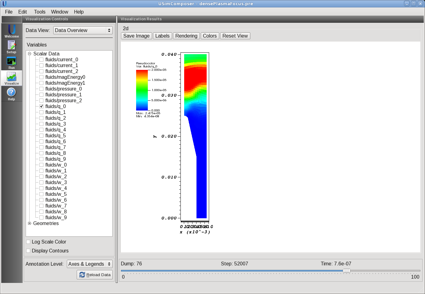
• Expand Scalar Data and click the check box for fluids/q_0 to visualize the mass density of the plasma.
• Drag the slider at the bottom of the Visualization Results pane to move through the simulation in time. The results near the end of the simulation are shown in Fig. 85.

Figure 85: Visualization of mass density in the Dense Plasma Focus example

Further experiments¶

Two ExodusII format mesh files are included with this example. The default file choice is “dpf.g”, which is a mesh partitioned for serial execution. Additional meshes (dpf.g.2.*, dpf.g.4.*, dpf.g.8.*) are included for 2, 4, and 8 core runs, respectively. Unlike GMSH meshes, it is not necessary to specify the number of cores that the mesh is partioned onto; USim looks for the appropriate files automatically. To run the example using the 2-core mesh, proceed as follows:

• Return to the Run window by pressing the Run icon in the workflow panel.
• In the Run window, press the MPI tab in the Runtime Options pane.
• Check the box marked Run with MPI and set Number of Cores equal to 2.
• To run the simulation, click on the Run button in the upper right corner of the Logs and Output Files pane. You will again see the engine output in the Logs and Output Files pane`.

After the simulation has executed, continue as follows:

• Proceed to the Visualize window as instructed by pressing the Visualize icon in the workflow panel.
• Press the Open button to begin visualizing.
• Expand Geometries in the Visualization Controls pane and click the checkbox for fluids/domain to visualize simulation geometry.
• Expand Scalar Data and click the check box for fluids/q_0 to visualize fluid densities.
• Drag the slider at the bottom of the Visualization Results pane to move through the simulation in time.

We can run further experiments on the dense plasma focus. For example, we can explore the effect of increasing the current (CURRENT) or decreasing the number density (N0). In the latter case, the plasma should move faster.