Using USim to Solve Navier-Stokes Equations
Conservative form of Navier-Stokes equations are solved in USim. Convective and diffusion terms are de-coupled. Hence the diffusion terms are added as source in the Euler equations (see Using USim to solve the Euler Equations).
Contents
Evaluation and Addition of the Diffusion Terms
The Updater block is evaluated in the time integration multiUpdater of the input file. Again referring to Supersonic cross flow over cylinder example of the USimHS package, the following updater block is used for time integration of fluxes using first order Runge-Kutta method. In this multiUpdater, computeViscousFluxes is added to the list of the updaters (updaters = [.,.,.,.,.]) to evaluate diffusion fluxes.:
<Updater rkUpdaterMain>
  kind = multiUpdater2d
  onGrid = domain

  in = [q]
  out = [qnew]

  <TimeIntegrator rkIntegrator>
    kind = rungeKutta2d
    ongrid = domain
    scheme = first
  </TimeIntegrator>

  <UpdateSequence sequence>
    loop = [boundaries,compute,hyper]
  </UpdateSequence>

  <UpdateStep boundaries>
     updaters = [correct, bcBottom, bcTop, bcRight, bcWall, bcLeft, computeT, bcWallTemp]
     syncVars = [q]
  </UpdateStep>

  <UpdateStep compute>
  operation = "operate"
     updaters = [computeVelocity, computeViscosity, computeKinematicViscosity, computeThermalCoefficient, \
                 computeThermalDiffusivity, computeViscousFluxes]
     syncVars = [source]
  </UpdateStep>

  <UpdateStep hyper>
     operation = "integrate"
     updaters = [hyper,addSource]
     syncVars = [qnew]
  </UpdateStep>

</Updater>
| option: | kind (string) |
|---|
name of of the this time integration updater multiUpdater2d (2d for two dimensional space).
| option: | in (nodalArray) variables to be integrated in time. |
|---|---|
| option: | out (nodalArray) name of the output variable. |
| option: | TimeIntegrator (sub block) type of integration scheme is rungeKutta2d with first order scheme. |
| option: | UpdateSequence (sub block) specifies the suquence loop of UpdateSteps. |
| option: | UpdateStep (sub blocks) Consists of the names of the user defined updater blocks required to be evaluated during the time integration steps. Note that, the names are user-given in the inputfile. And the order of evaluation is important. |
correct, bcBottom, bcTop, bcRight, bcWall, bcLeft, computeT, bcWallTemp, computeVelocity, computeViscosity, computeKinematicViscosity, computeThermalCoefficient, computeThermalDiffusivity, are the other updater blocks to evaluate and apply boundary conditions and thermophysical properties. These updater blocks are found in the Supersonic cross flow over cylinder example. Their usefulness will be briefed here in this lesson. correct corrects the values of any variables of interest to user specified limits. bcBottom, bcTop, bcRight, bcWall, bcLeft are the boundary conditions for conservative variables (here in this example, they are mass, three components of momentum, and energy density). computeT is for obtaining temperature from the conservative variables. bcWallTemp applies user specified temperature on the wall. ‘computeVelocity’ obtains the velocity from the conservative variables. computeViscosity, computeKinematicViscosity, computeThermalCoefficient, computeThermalDiffusivity are updater blocks used to compute thermophysical properties varying with temperature. Note that these blocks can be eliminated from the input file, if the properties are constant. computeViscousFluxes evaluates the viscous and thermal fluxes using the updater block shown above. hyper is classicMuscl updater block used to evaluate the convective fluxes from the hyperbolic part of the NS equations. Now the diffusion source is added to the existing convective sources using the combiner2d updater as shown below:
<Updater addSource>
  kind = combiner2d
  onGrid = domain
  in = [qnew, source]
  out = [qnew]
  indVars_qnew = ["rho", "mx", "my", "mz", "en"]
  indVars_source = ["sx","sy","sz","sen"]
  exprs = ["rho","mx+sx","my+sy","mz+sz","en+sen"]
</Updater>
| option: | syncVars_computeViscousFluxes (optional attribute) This option synchronizes the diffusion fluxes in the variable source. All of the computed variables which need information from the cells in the adjacent partition (used in parallel computing) have to be synchronized using this option. Differentiation operators are used in computeViscousFluxes and the result is stored in source. Hence source is synChronized after calling computeViscousFluxes. |
|---|---|
| option: | syncVars_bcRight (optional attribute) used for the same reason as specified above. |
| option: | dummyVariables_q The dummy variables qDummy1, qDummy2, qDummy3 are required for Runge-Kutta integration. Each of the integration variable should have a different dummyVariables_ = [.,.,.] option. |
| option: | syncAfterSubStep qnew which has the updated values of the integration is synchronized at the end of integration. |
Time Step Restriction
Time step restriction has to be added separately for hyperbolic and elliptic terms. The following three restriction are evaluated and added in the loop.
Hyperbolic restriction:
 <Updater timeStepRestriction>
   kind = timeStepRestrictionUpdater2d
   in = [q]
   onGrid = domain
   restrictions = [hyperbolic]
   <TimeStepRestriction hyperbolic>
     kind = hyperbolic
     model = eulerEqn
     cfl = CFL
     gasGamma = GAS_GAMMA
   </TimeStepRestriction>
</Updater>
Viscous diffusion time step restriction:
<Updater timeStepRestriction2>
  kind = timeStepRestrictionUpdater2d
  in = [kinematicViscosity]
  onGrid = domain
  restrictions = [quadratic]

  <TimeStepRestriction quadratic>
    kind = quadratic
    cfl = 0.5
  </TimeStepRestriction>
</Updater>
Thermal diffusion time step restriction:
 <Updater timeStepRestriction3>
   kind = timeStepRestrictionUpdater2d
   in = [thermalDiffusivity]
   onGrid = domain
   restrictions = [quadratic]
  <TimeStepRestriction quadratic>
    kind = quadratic
    cfl = 0.5
  </TimeStepRestriction>
</Updater>
In all of the above time step restrictions, cfl can be varied according to the problem.
An Example Simulation
The Supersonic cross flow over cylinder example of the USimHS demonstrates each of the concepts described above. Executing the Supersonic cross flow over cylinder input file within USimComposer and switching to the Visualize tab yields the plot shown in Fig. 7.
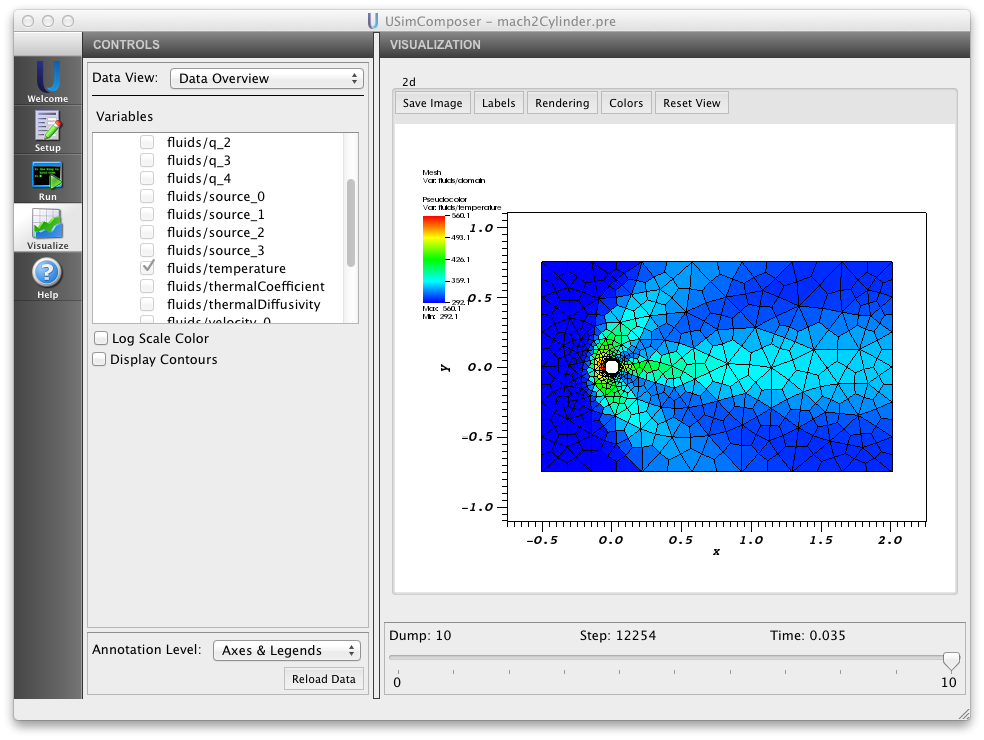
Figure 7: Visualization tab in USimComposer after executing the input file for the tutorial.