Geometric Biasing

Problem Description

This example is designed to show how the geometric biasing feature of RSim functions with a simple theoretical problem. Geometric biasing works by creating a number of computational spheres in the simulation space, moving inwards from a standard spherical particle source to a defined innermost sphere. The number of spheres is selected by the user. As a particle crosses into a sphere, its weight will be cut in half and the number of particles doubled. This can be used to improve statistics in shielding problems, when large numbers of particles may be absorbed by the shield.

Opening the Simulation

The Geometric Biasing example is accessed from within RSim by the following actions:

• Select the New → From Example… menu item in the File menu.
• In the resulting Examples window expand the RSim for Basic Radiation option.
• Expand the Basic Examples option.
• Select Geometric Biasing and press the Choose button.
• In the resulting dialog, create a New Folder if desired, and press the Save button to create a copy of this example.

All of the properties and values that create the simulation are now available in the Setup Window as shown in Fig. 57. You can expand the tree elements and navigate through the various properties, making any changes you desire. The right pane shows a 3D view of the geometry, if any, as well as the grid, if actively shown.

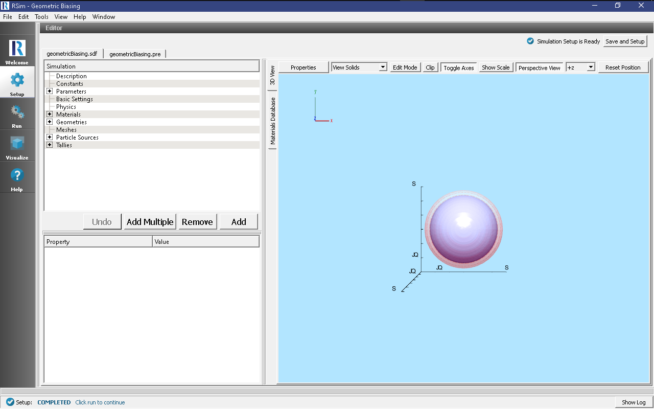
Fig. 57 Setup Window for the Geometric Biasing example.

Simulation Properties

For this example 4 spherical shells are created, spaced at 1 meter increments between a radius of 1 and 4 meters. The shells themselves are of galactic material, so as to not impact the simulation.

A particle source is created, which makes use of the geantino particle. These are not physical particles, but can be used for testing problem setups without a concern for the physics in question. It is a radius of 4.6 meters, with the sphere bias selected with inner radius of 0.5 meters. 5 bias layers are set, this will create one bias layer outside the largest shell, and then between each shell. A focused angular distribution is used, this will aim all particles at the center of particle source.

Two Number of Track tallies have been added for each shell, one that will weight the results, and one that will not. This will track the number of particles that pass through each shell. Since we are using geantino’s we do not have to be concerned with a particle losing energy in any shell, and the number of particles will be consistent for each shell.

Running the Simulation

After performing the above actions, continue as follows:

• Proceed to the Run Window by pressing the Run button in the left column of buttons.
• To run the file, click on the Run button in the upper left corner of the Logs and Output Files pane. You will see the output of the run in the right pane. The run has completed when you see the output, “Engine completed successfully.” This is shown in Fig. 58.

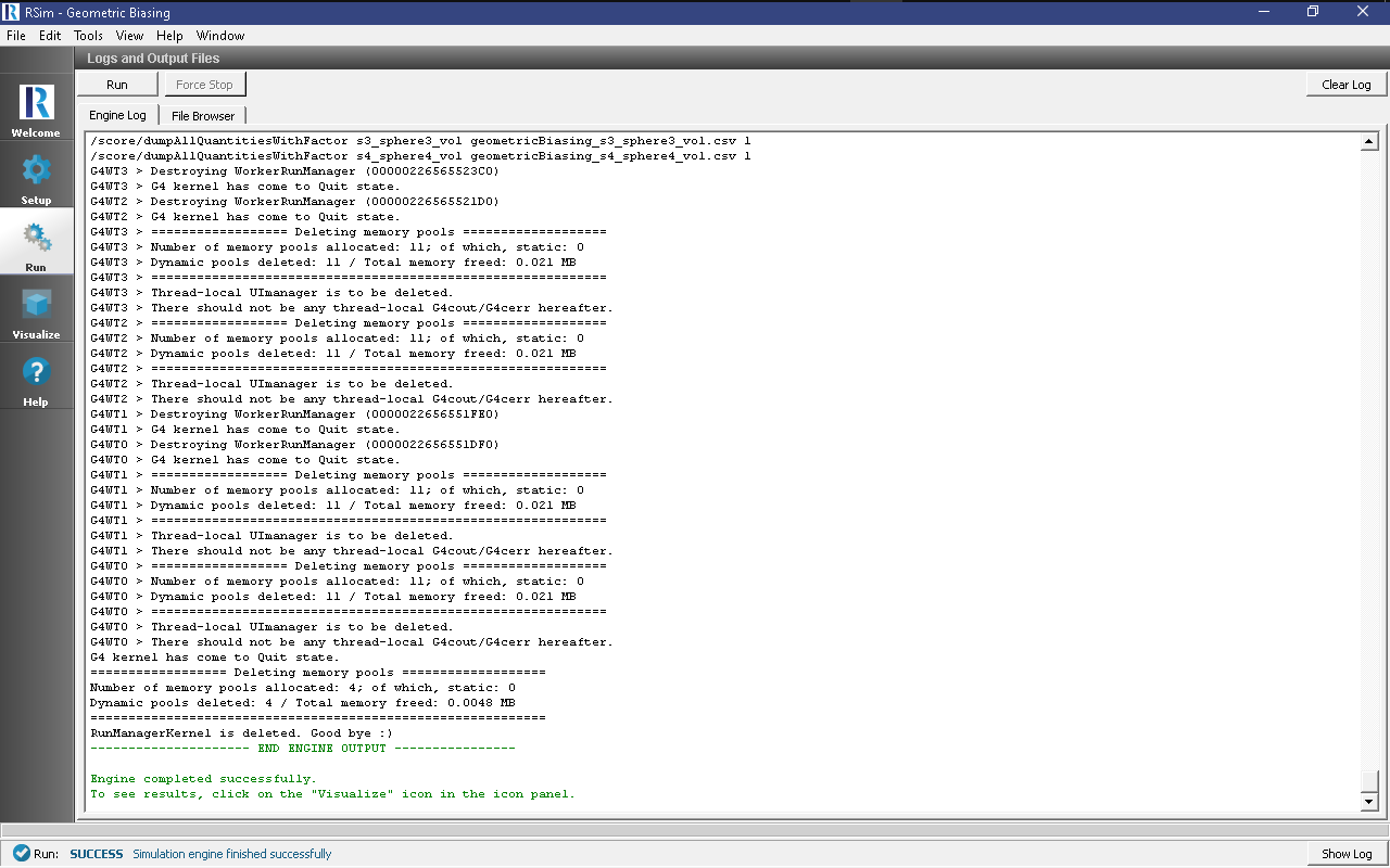
Fig. 58 The Run Window at the end of execution.

Visualizing the Results

After the run has completed the results of all tallies can be compared. For this example it is best to look at the number of tracks, which have been recorded in both a weighted and unweighted form.

The results for the * Expand Scalar Data * Select NumberOfTrackSphere1 * Select NumberOfTrackSphere2 * Select NumberOfTrackSphere3 * Select NumberOfTrackSphere4 * Select Clip Plot from the Scalar Data selection (as shown in figure 59) to apply to all data selections

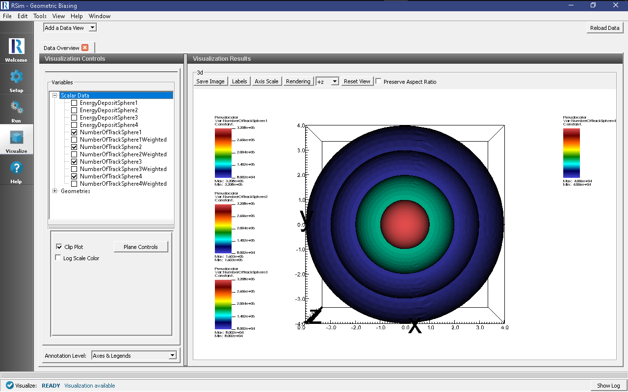
Fig. 59 A visualization of the number of tracks

Looking at these results, we can see the number of tracks in sphere 4 is 4e4. This doubles in track 3 to 8e4, again in sphere2 at 1.596e5, and again to sphere 1 at 3.198e5. This performs exactly as expected. To see the fact that the weights are cut in half for each track, repeat the procedure with the weighted tallies, we see all tallies are nearly identical between 1.995e4 and 2.004e4

Further Experiments

Try adjusting the materials from galactic to aluminum, to see how this improve statistics on inner spheres as particles get absorbed on outer spheres.