Smith-Purcell Radiation (SmithPurcellRadiation.sdf)

Keywords:

diffraction grating, radiation generation, coherent mode, Smith-Purcell

Warning

This example used more than 8GB of RAM as configured, so if your machine does not have a lot of memory, then you can reduce the number of cells in the Grid (say by a factor of 2 to the size 950x800x2) to avoid running out of memory.

Problem Description

This VSim for Vacuum Electronics example illustrates how to setup a device that emits coherent Smith-Purcell Radiation (SPR). This phenomenon occurs when charged particles pass over a periodically graded surface in very close proximity resulting in the emission of a form of Cherenkov radiation. In recent years, engineers have been building SPR-emitting devices that can generate frequencies in the terahertz range, otherwise difficult to obtain via other methods. This example demonstrates how the design of an SPR-emitting device can be optimized with simulations.

This simulation can be run with a VSimVE license.

Opening the Simulation

The Smith-Purcell Radiation example is accessed from within VSimComposer by the following actions:

Select the New → From Example… menu item in the File menu.
In the resulting Examples window expand the VSim for Vacuum Electronics option.
Expand the Radiation Generation option.
Select Smith-Purcell Radiation and press the Choose button.
In the resulting dialog, create a New Folder if desired, then press the Save button to create a copy of this example.
The resulting Setup Window is shown Fig. 394.

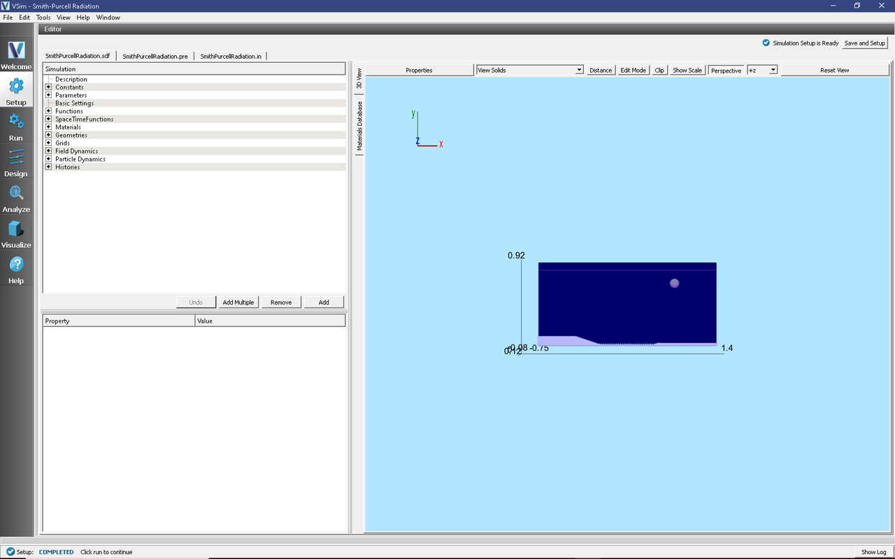
Fig. 394 Setup Window for the Smith-Purcell Radiation example.

Simulation Properties

The simulation setup was based on Donohue & Gardelle 2005 [DG05] who used 2D simulations for their study: a grating structure that is perfectly conducting, a cathode from which the electron beam is emitted, and a vacuum enclosure in which radiation propagates. The walls of the vacuum box are matched absorbing layers (MALs) which absorb the electromagnetic fields and eliminate any reflection. This is a quasi-3D simulation: the thickness to the gating structure is 2cm and the simulation is periodic in z (the direction normal to the grating). The grid resolution was set high enough to resolve the small structures of the grating: 1890, 1600, and 2 cells in the x, y, and z directions, respectively. The 5 mm electron beam was generated with a 125 A/m current. The incident electron energy is 100 keV. There is an external magnetic field of 2 T in the x-direction for beam confinement.

Running the Simulation

Once finished with the setup, continue as follows:

Proceed to the Run Window by pressing the Run button in the navigation column out left.
To run the file, click on the Run button in the upper left corner of the Logs and Output Files pane. You will see the output of the run in that pane. The run has completed successfully when you see the output, “Engine completed successfully.” This is shown in Fig. 395.

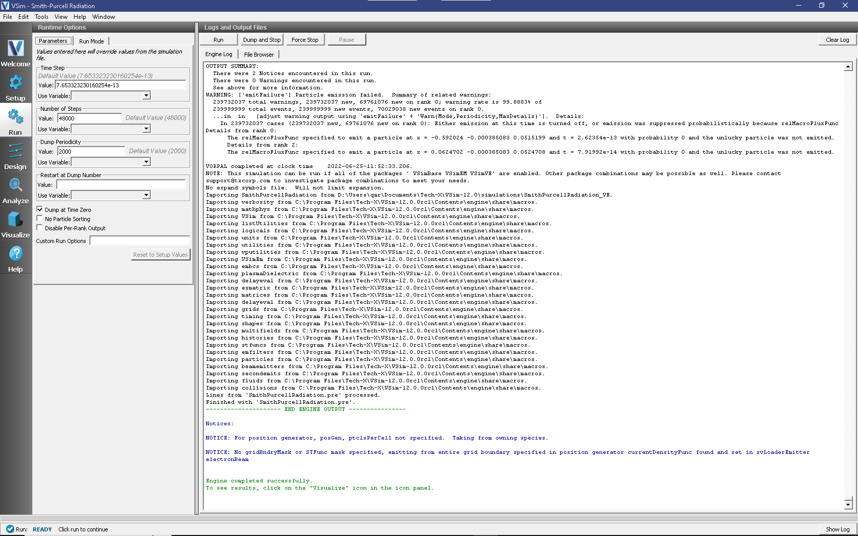
Fig. 395 The Run Window at the end of execution.

Visualizing the Results

After performing the above actions, the results can be visualized as follows:

Proceed to the Visualize Window by pressing the Visualize button in the navigation column.
From the Data View dropdown menu, select Data Overview.
In the variables tree, expand Scalar Data.
Expand B.
Select B_z.
Check Set Minimum and Set Maximum and set to -1e-5 and 1e-5, respectively
In the bottom of the right pane, mode the dump slide forward in time.
The resulting visualization is shown in Fig. 396.

Fig. 396 Bz at the end at 25 ns (at dump 24).

The magnetic field in the z direction (Bz) plotted in Fig. 396 shows that at 85 cm and 64 degrees from the center of the grading the SPR emission was the strongest (this is known as the SPR propagating mode). This is consisted with the results found by Donohoe and Gardelle. The strong emission seen on the left side is known as the evanescent mode, but this is considered non-SPR emission.

To measure the frequencies of these modes proceed as follows:

Proceed to the Visualize Window by pressing the Visualize button in the navigation column.
From the Data View dropdown menu, select History.
Select Bz64deg_2 from the drop-down menu in Graph 1.
Select None for Graphs 2,3, and 4.
In the top left corner of the right pane, check the Fourier Amplitude (dB) option.
In the upper right corner of each plot, select Limits and set X-Axis max to 1.2e10 and click OK.
The resulting visualization is shown in Fig. 397.

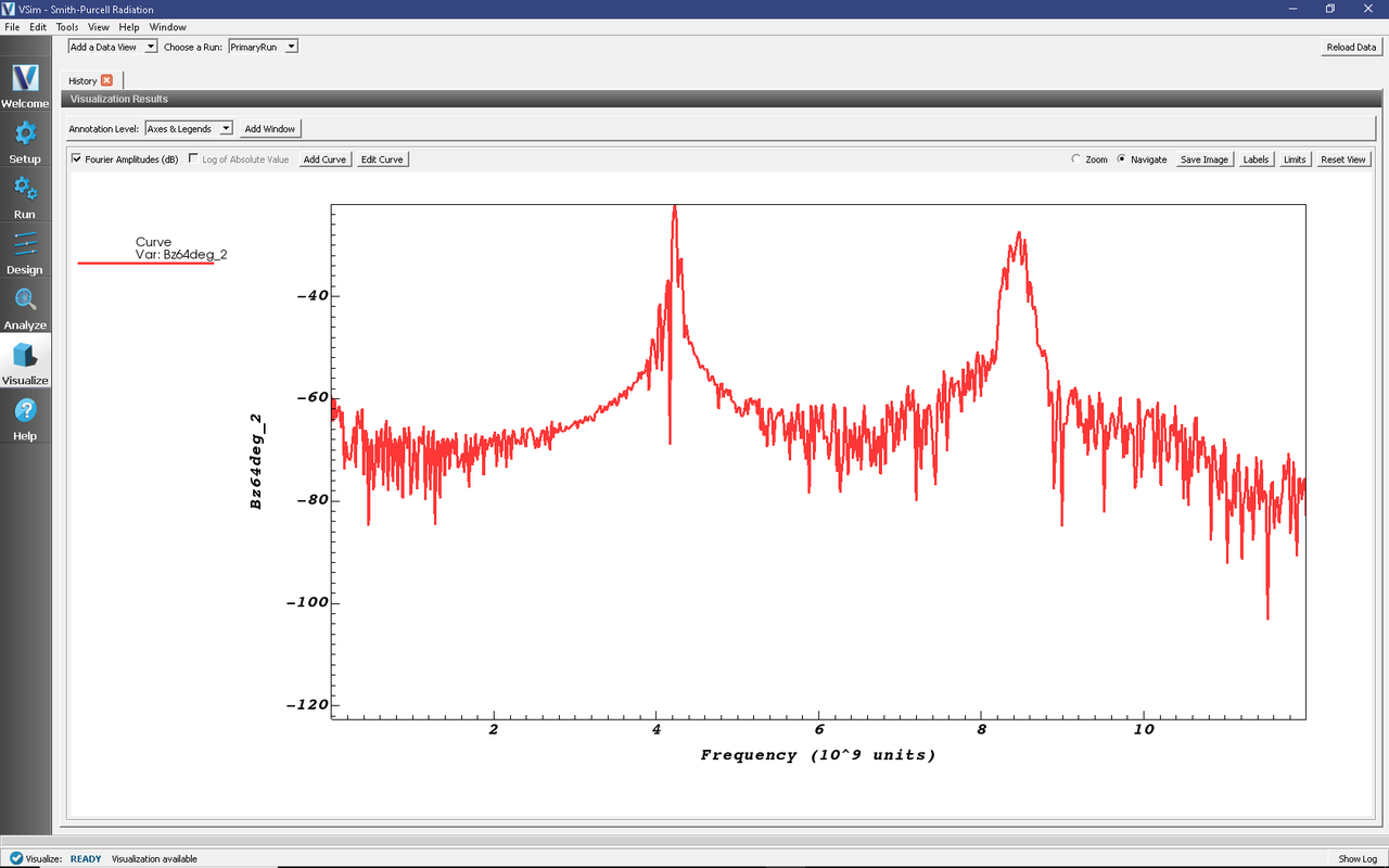
Fig. 397 FFT of the Bz measured at 85 cm and 64 degrees from the center of the grading where the SPR emission was the strongest. The frequencies of the evanescent and the propagating modes can be seen at around 4.5 and 9 GHz.

The FFT of this signal is shown in Fig. 397 where the frequencies corresponding to the evanescent mode and the propagating mode can be seen at around 4.5 and 9 GHz. The evanescent mode becomes dominant over the propagating mode when the dampers are not present. Note: it is expected for the propagating mode frequency to be an integer multiple of the evanescent mode (see Donohue and Gardelle 2005 [DG05] for more details).

Another signature of SPR emission is electron bunching inside the particle beam. To visualize the electron bunching, proceed as follows:

Proceed to the Visualize Window by pressing the Visualize button in the navigation column.
From the Data View dropdown menu, select Phase Space.
For the X-axis, select electrons_x.
For the Y-axis, select electrons_ux.
Click Draw.
Move the dump slider further in time.
The resulting visualization is shown in Fig. 398.

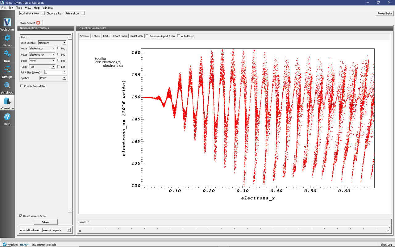
Fig. 398 The phase-space visualization for the Smith-Purcell Radiation example.

Fig. 398 shows a phase-space of the electron speed in the propagation direction vs. their position. The very strong bunching effect can be observed and this effect becomes more defined and increases with time.

Further Experiments

When running the simulation without the dampers, the evanescent mode is dominant and strong fields can be seen at the beginning and end of the electron beam. Adding wedge-like dielectric structures can help damp the strong non-SPR beam. Further extension of the cathode damper and adjusting the dielectric constant makes the SPR beam became dominant as show in this simulation. The dielectric dampers are critical in obtaining a strong SPR emission.

Using this basic setup, one can develop a simulation for special SPR emission which is generally obtained by narrowing the grooves inside the grating.