Gyrotron Mode (gyrotronMode.sdf)

Keywords:

gyrotron

Problem description

This VSimVE example illustrates a very high order mode, TE-22-6, propagating in a cylindrical waveguide, very near to the cutoff frequency, which is a common situation in a gyrotron. The example is intended to allow investigation of the axial phase and group velocity of such a mode, as a function of frequency, and to highlight the intricacies of simulating a mode that is propagating within a percent or two of its cutoff frequency.

This simulation can be performed with a VSimVE license.

Opening the Simulation

The Gyrotron Mode example is accessed from within VSimComposer by the following actions:

• Select the New → From Example… menu item in the File menu.

• In the resulting Examples window expand the VSim for Vacuum Electronics option.

• Expand the Radiation Generation option.

• Select “Gyrotron Mode” and press the Choose button.

• In the resulting dialog, create a New Folder if desired, and press the Save button to create a copy of this example.

The Setup Window is now shown with all the implemented physics and geometries, if applicable. See Fig. 415.

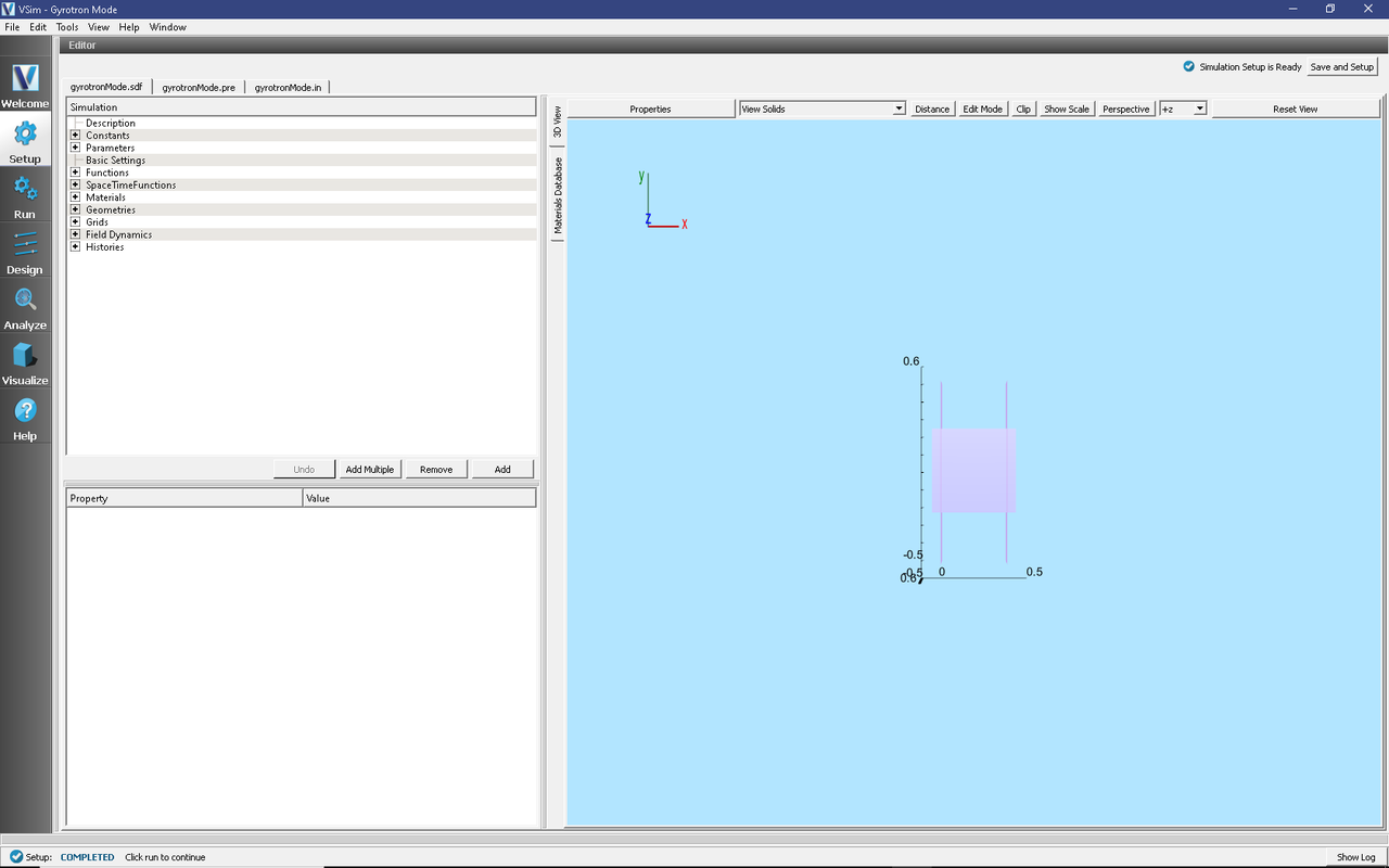
Fig. 415 Setup Window for the Gyrotron Mode example.

The basic variables of this problem should now be alterable via the text boxes in the left pane of the Setup Window, as shown in Fig. 415.

Simulation Properties

There are only two geometrical input parameters; the waveguide radius and length. The user may also control the excitation frequency, the duration of the simulation, and the nature of the excitation, specifically whether it is pulsed or continuous-wave. Additional exposed parameters include the grid sizes, and the tuning of the exiting wave boundary condition, which allows for more in-depth study with this example.

The excitation may be pulsed or continuous-wave, depending on the current input values in the element tree under Field Dynamics → Current Distributions → distributedCurrent0. The default J_y and J_z values are driveOffEy and driveOffEz, respectively, for a pulsed driver. The user can change these values to driveOnEy and driveOnEz for a continuous driver. The two methods of driving the cavity are described in the following.

Pulsed Simulation (driveOffE)

In this case, the wave is driven for half of the simulation duration, with a smooth turn-on / turn-off time window. Then, for the remaining half of the periods, the excitation propagates freely. The axial profile of the pulse will be very short, typically just one or two axial wavelengths. It will propagate slowly down the waveguide, as expected from the group velocity which is very small near cutoff. In the center of the pulse the TE-22-6 mode is preserved, but because this is a pulse, nearby modes in frequency are also present. One can observe a rich set of other mode patterns just a few grid planes away from the center of the pulse.

Continuous-Wave Simulation (driveOnE)

The drive may be kept on, instead of having it turn off halfway through the simulation. After an initial transient, this sets up a single TE-22-6 traveling wave mode pattern throughout the waveguide. This allows for accurate measurement of the axial wavenumber, beta, for the mode.

Running the simulation

After performing the above actions, continue as follows:

• Proceed to the run window by pressing the Run button in the left column of buttons.

• To run the file, click on the Run button in the upper left corner of the right panel. You will see the output of the run in the right pane. The run has completed when you see the output, “Engine completed successfully.” This is shown in Fig. 416.

Fig. 416 The Run Window at the end of execution.

Visualizing the results

After performing the above actions, continue as follows:

• Proceed to the Visualize Window by pressing the Visualize button in the left column of buttons.

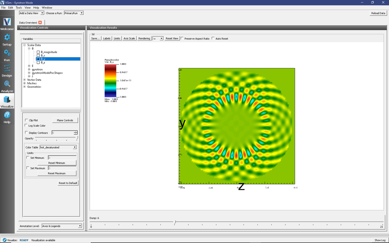
Fig. 417 Illustration of the mode pattern, and propagation of the mode down the length of the tube.

The \(B_x\) field is the best component for looking at in this simulation, as shown in Fig. 417.

• Expand Scalar Data.

• Expand B

• Select B_x

• Using the cursor, grab the image and rotate it from right to left by 90 degrees.

• Move the dump slider to dump 11.

The initial parameters are selected so that the excitation frequency is just barely above cutoff. While the axial phase velocity is high in this case, the group velocity is quite low, and the simulation shows a narrow wavepacket slowly moving down the length of the tube, while remarkably still maintaining the very high order TE-22-6 pattern. Contamination of the pattern increases as the duration of the excitation is reduced, since more frequencies are brought into the transient. The user is encouraged to look at the mode pattern and contamination properties as frequency and duration are varied.

The TE-22-6 mode’s cutoff frequency, for the suggested initial radius of 20 cm, is known analytically to be 10.8845 GHz, which derives from the value of the 6th root of the \(J_{22}\) bessel function, which is 45.624312. However, the user will note that the suggested initial drive frequency is below this, at 10.74 GHz, and yet the wave appears to propagate! This illustrates an important property of finite-difference dispersion, that in fact the speed of light is ever-so-slightly slower in the finite-difference-time-domain simulation than in reality. In most cases, this is hardly noticed, however, when operating this close to the cutoff frequency of a waveguide, this difference can be readily seen, as this example illustrates. The discrepancy between the discrete FDTD cutoff frequency and the analytic cutoff frequency, depends on the grid resolution of the wave, and in general decreases as \(\delta x^2\), where \(\delta x\) is the grid size.

A very useful piece of information is the FDTD cutoff frequency. This may be found with a series of simulations, each at different drive frequencies, \(\omega\). The KEEP_DRIVE_ON parameter should be set to 1, so that the axial wavelength, \(\beta\), can be measured from the field plots. A plot of \(\omega^2\) vs. \(\beta^2\) should be essentially linear, with the intercept on the \(\omega^2\) axis being the FDTD cutoff frequency, \(\omega_{cutoff}^2\) (\(\omega^2 = \omega_{cutoff}^2 + c^2 \beta^2\)), and with slope being the FDTD speed-of-light-squared. A spreadsheet showing this exercise for the suggested initial values of the example is shown below. The result of this study is that the FDTD cutoff frequency is actually 10.675 GHz, or 2% below the known analytical result, for the initial suggested grid resolution.

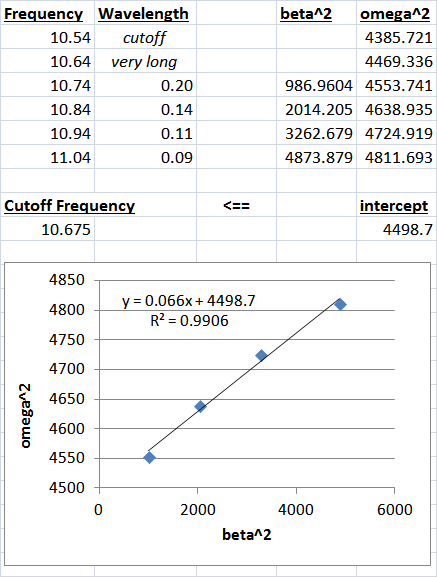
Fig. 418 Computing the FDTD cutoff frequency of the TE-22-6 mode.

Further Experiments

The user is encouraged to repeat the simulations discussed in the previous section with a finer resolution, to see how the FDTD cutoff frequency approaches the analytic result as resolution improves.

The detailed TE-22-6 mode pattern is very carefully crafted using polynomial fitting functions, and is introduced into the axial magnetic field, \(B_x\), at the left side of the simulation. There is no direct option to use a different mode, although the user may attempt to edit the detail of the input to do so.

Finally, a boundary condition tuning parameter, VPHASE_PORT, is offered to allow the user to experiment with tuning of the outgoing wave boundary condition in this near cutoff scenario. In this circumstance, the optimal phase velocity may be 5 to 10 times the speed of light.

An additional exposed user parameter, FREQ_CUTOFF, is offered, and may be used to store the value derived from the simulations discussed in the previous section. By default, this parameter is not used. However the user may look into the detail of input file, and notice a comment line that indicates how this parameter might be used to set the value of VPHASE_PORT more accurately.