Helix Traveling Wave Tube 1: Dispersion (helixTwt1Dispersion.sdf)
Keywords:
- Helix TWT Dispersion Analysis Run
Problem description
This VSimVE example is one of a set of simulations showing different calculations to aid the design of a helix traveling wave tube (TWT) in three dimensions. The 100-turn helix with end feeds is imported from a CAD file, but all other geometrical parts are created with the Constructive Solid Geometry (CSG) capabilities within VSimComposer. The dependence of the geometries on the constants and parameters will be discussed in Helix Traveling Wave Tube 2: Impedance and Attenuation (helixTwt2ImpedAtten.sdf).
This simulation addresses the dispersion analysis of the tube and as such runs with a grid covering a reduced number of helix turns. An impulse signal is excited between the helix and the body tube (which would be the vacuum interface in a real device) and periodic boundary conditions are enforced at the two ends. The tube is allowed to run for sufficiently long to observe the behavior at relatively low frequencies. We are able to recover the phase velocity of the wave on the helix (and so the structure/RF curve on an omega beta diagram) from this simulation. It differs from the other simulations of helix TWT in that the simulated region contains no coaxial coupler. As well the attenuator is outside the simulated region. For other studies of the TWT, see
This simulation can be performed with a VSimVE or VSimPD license.
Opening the Simulation
The Helix TWT example is accessed from within VSimComposer by the following actions:
Select the New → From Example… menu item in the File menu.
In the resulting Examples window expand the VSim for Vacuum Electronics option.
Expand the Radiation Generation option.
Select “Helix Traveling Wave Tube 1: Dispersion” and press the Choose button.
In the resulting dialog, create a New Folder if desired, and press the Save button to create a copy of this example.
All of the properties and values that create the simulation are
now available in the Setup Window as shown in
Fig. 419. The right pane shows a
3D view of the geometry, if any, as well as the grid, if actively
shown. To show or hide the grid, expand the Grid element and
select or deselect the box next to Grid.
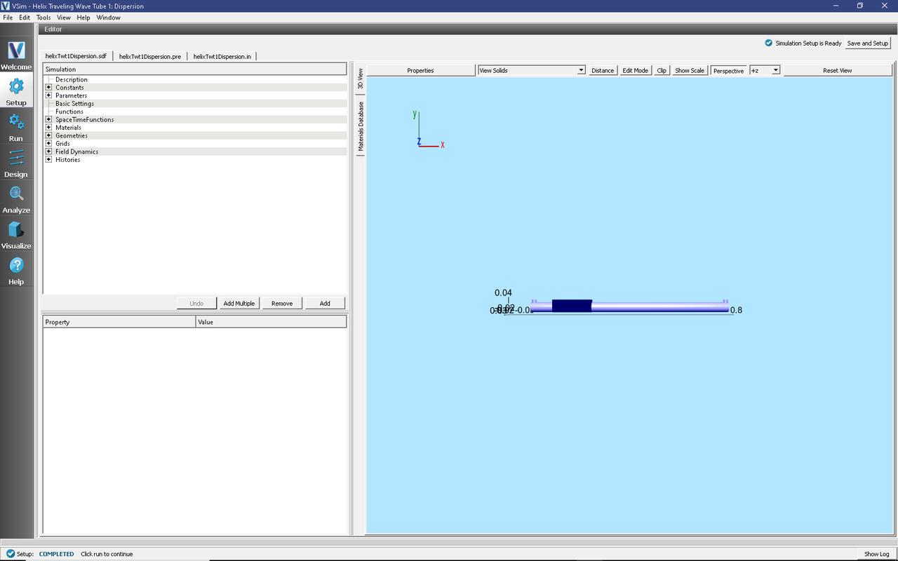
Fig. 419 Setup Window for the Helix TWT example.
The geometry of the helix can be made more visible by unselecting the tube and emitter disk parts under Geometries/CSG in the tree (e.g. driftTubeSolid, tubeSolid, driftTubeVoid, tubeVoid, tube, and emitterDisk) or by changing their color property and selecting a low alpha on Windows or Linux (or opacity on Mac). See color property setting in the User Guide.
setting is made available by clicking on the “Properties” button.
Running the simulation
After performing the above actions, continue as follows:
Proceed to the run window by pressing the Run button in the left column of buttons.
To run the file, click on the Run button in the upper left corner of the right panel. You will see the output of the run in the right pane. The run has completed when you see the output, “Engine completed successfully.” This is shown in Fig. 420.
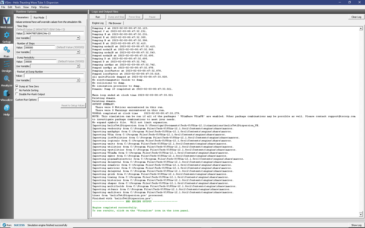
Fig. 420 The Run Window at the end of execution.
The simulation allows a frequency domain analysis to be performed. In order to resolve low frequency signals, a large number of steps is required. Increasing the number of steps further may help to improve the frequency domain resolution, especially at the low frequency end of the spectrum. The Dump Periodicity may be increased to reduce the number of data dumps and save space at the expense of being able to view up to date simulation data while it runs.
Visualizing the results
After performing the above actions, continue as follows:
Proceed to the Visualize Window by pressing the Visualize button in the left column of buttons.
To see the fields inside the tube as shown in Fig. 421, do the following:
Expand Scalar Data
Expand E
Select E_x
Select the Clip Plot checkbox
Select the Set Minimum checkbox and set to -0.05
Select the Set Maximum checkbox and set to 0.05
Select the Display Contours checkbox and set # of contours to 4.
Expand Geometries
Select poly (helixTwtWithFeedsGeomSolid)
Click the Clip Plot checkbox
Move the dump slider forward in time to see the evolution
Click and drag to rotate the image
The wave travels along the helix, and the strongest fields occur between turns. The individual modes are not separated out in this case.
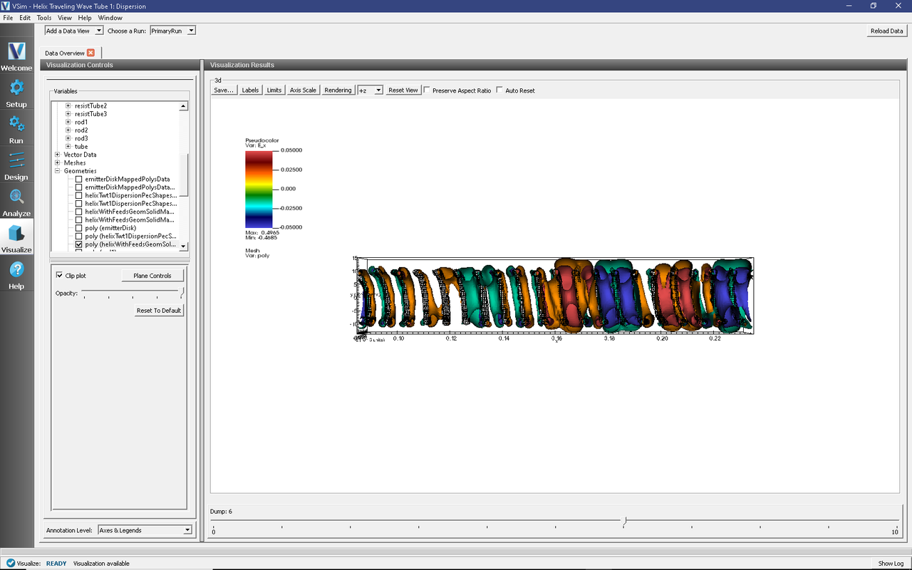
Fig. 421 Longitudinal field, E_x, for the dispersion run at time step 120,000.
The History records can be used to calculate the dispersion curve:
Select the Add A Data View dropdown menu and click History
Set EonAxisA_0 under Graph 1
Set EonAxisA_1 under Graph 2
Under Graph 3 and Graph 4 change the dataset to <None>
Check “Fourier Amplitudes (dB)” button at top left of plot
Select Zoom radio button
Using the Limits button above the plot set both to have limits of 0 to 2e9.
The result is shown in Fig. 422 (to which we have added vertical measuring lines using an external image editing software). A series of peaks can be seen. The mode frequencies correspond to the maxima of this plot. Having more than one history is important as due to mode variation in space, one history may pick up modes another misses and vice-versa.
Record the frequencies at which these peaks occur, e.g. in a spreadsheet. With the view mode switched from Zoom to Navigate, a wheel mouse can be scrolled up and down to zoom in and out. This may expedite the process of collecting the data. Or, as we have done, one can add vertical measuring lines after opening the image in some external software.
The first seven frequencies from the 300000 step simulation are listed in the table below. To determine the phase velocity \(v_n\) for each mode frequency, first note that the wave number for the \(n\)-th mode is given by
where L is the length of the helix TWT. The phase velocity for the \(n\)-th mode is then
where \(f_n\) is the frequency of the \(n\)-th mode and c is the speed of light. The first 10 mode phase velocities are listed in the table below for \(L\) = 15 cm. For large frequencies, we should expect the phase velocity to approach the ratio of the helix pitch (0.75 cm) to the circumference (6.28 cm), or 0.119.
n |
frequency (GHz) |
phase velocity (c) |
|---|---|---|
1 |
0.285 |
0.1425 |
2 |
0.555 |
0.1387 |
3 |
0.810 |
0.1350 |
4 |
1.048 |
0.1310 |
5 |
1.285 |
0.1285 |
6 |
1.520 |
0.1267 |
7 |
1.770 |
0.1264 |
Higher resolution and longer duration simulation could be used to better measure the frequencies and, hence, determine the phase velocity. Even more precise frequencies could be obtained by the Filter Diagonalization Method.
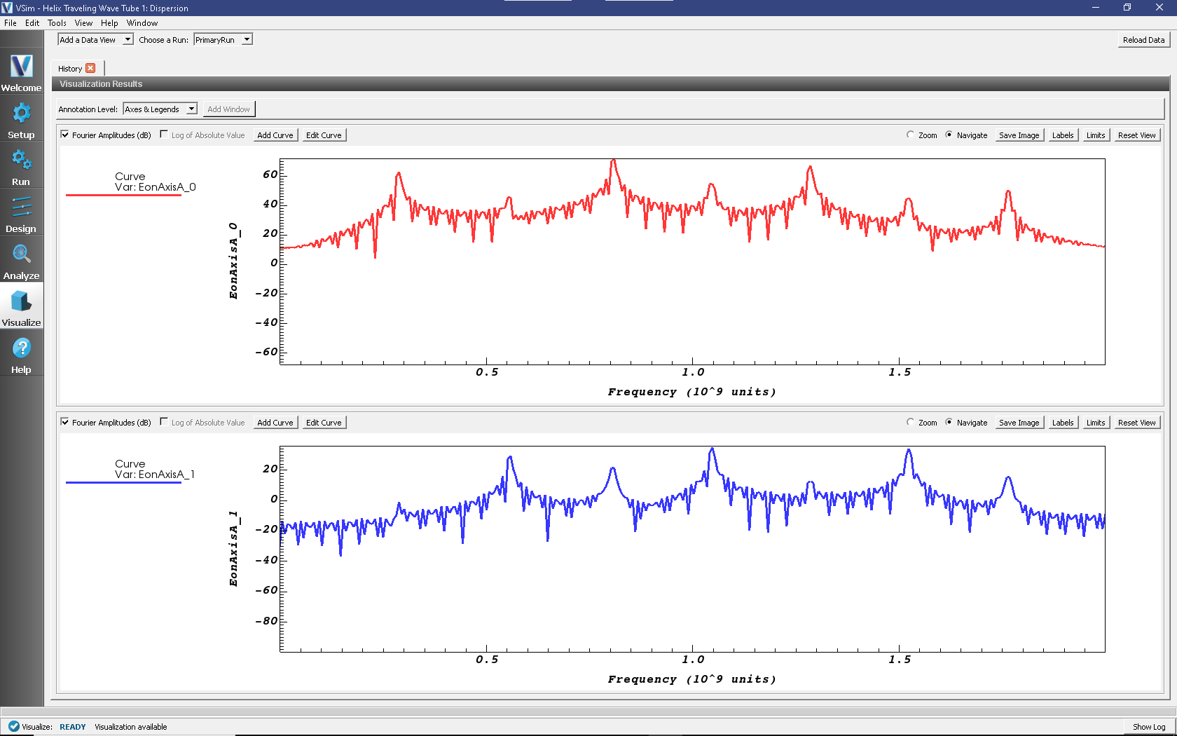
Fig. 422 Fourier transform of various histories after 300000 timesteps.
Further tests
The axial phase velocity is chosen to be synchronous with the beam. Adjust the helix parameters (in an external CAD editor) and observe the changes to the phase velocity.
Restarting after the default 300000 steps allows more accurate definition of the frequencies.
Use the Filter Diagonalization Method to get the frequencies more precisely.