Stairstep Cavity in coordinateGrid (emCavityCoordProdT.pre)
Keywords:
- stairstep boundary, coordinateGrid, Klystron cavity
Problem description
This example demonstrates how to set up a complex geometry
structure in VSim that uses the coordinateGrid system for
a varying mesh size. There are two benefits of constructing
a grid of kind coordProdGrid via coordinateGrid
blocks. The first is a flexible choice of either Cartesian
\((x,y,z)\) or cylindrical \((z,r,\phi)\) coordinate
systems to construct the grid. The second is that it enables
one to vary the cell size along each axis of the grid.
For example, a fine grid resolution can be used in a region
of the domain consisting of complicated geometry,
while a coarse resolution can be used in a different region
of the domain where the geometry is simple.
This method reduces the memory
requirement for large multiscale simulations.
The gridBoundary block (implemented in this example through
the geometry macro) is used by VSim to represent complex
geometrical surfaces with boundary conditions.
This example simulates a klystron cavity using a non-uniform Cartesian mesh generated by VSim’s coordinateGrid system. Klystron cavities have wide applications as RF power sources by amplifying an RF input with electron beams. The simulated cavity is defined by a set of VSim geometry macros. Grid cell size is varied in the longitudinal direction so that a fine mesh exists at the round nose surface connecting the center drifting tube and outer ring cavity. Larger cell sizes are used at both ends of the drifting tube. The fundamental transverse magnetic (TM) mode is excited by a Gaussian current pulse.
This simulation can be performed with either a VSimEM, VSimVE, or VSimPD license.
Opening the Simulation
The emCavityCoordProdT example is accessed from within VSimComposer by the following actions:
Select the New → From Example… menu item in the File menu.
In the resulting Examples window expand the VSim for Microwave Devices option.
Expand the Cavities and Waveguides (text-based setup) option.
Select “Stairstep Cavity in Coordinate Grid (text-based setup)” and press the Choose button.
In the resulting dialog, create a New Folder if desired, and press the Save button to create a copy of this example.
The basic variables of this problem should now be alterable via the text boxes in the left pane of the Setup Window, as shown in Fig. 389.
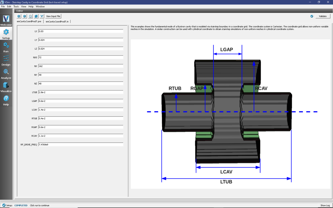
Fig. 389 Setup Window for the emCavityCoordProdT example.
Input File Features
At the top of the Editor pane, click View Input File.
The first important feature of this input file is the setup of the non-uniform simulation grid. Scroll to the Grid block on line 262 (Fig. 390). The variable spacing in \(x\) in the non-uniform grid is specified in the definitions of
sectionBreaks and deltaAtBreaks in the coordinateGrid dir0 block. The deltaAtBreaks field specifies the grid cell spacing at each of the sectionBreaks positions, and the grid is generated such that the cell spacing transitions gradually between these positions. In this specific example, on lines 266 and 267, from \(x=\) XBGN to \(x=\) CAV_START the cell spacing transitions from \(\Delta x=\) DX
to \(\Delta x=\) DX/3.0, then from \(x=\) CAV_START to \(x=\) CAV_END the cell spacing stays at a constant value of \(\Delta x=\) DX/3.0, and finally from \(x=\) CAV_END to \(x=\) XEND the cell spacing transitions from \(\Delta x=\) DX/3.0 back to \(\Delta x=\) DX.
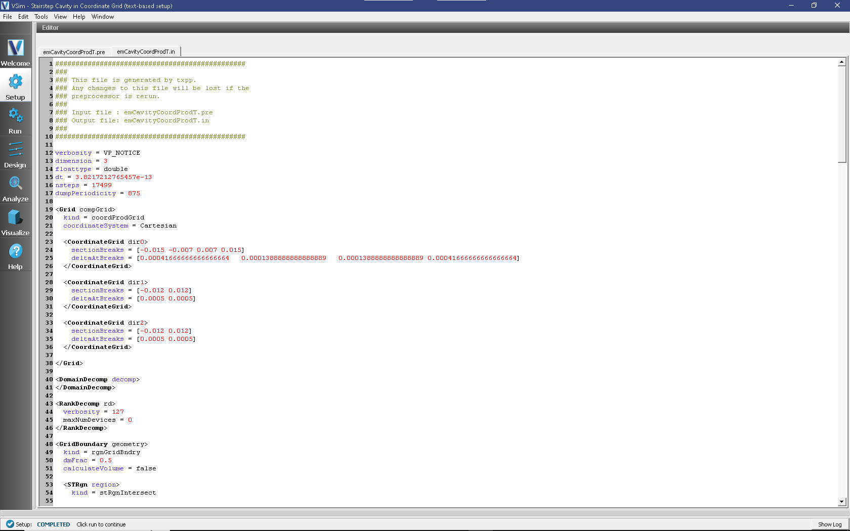
Fig. 390 Input file for the emCavityCoordProdT example, showing the setup of the coordinateGrid system.
The second important feature of this input file is
the electromagnetic solver for this type of grid. Both the Faraday and Ampere
updaters are set to kind curlUpdaterCoordProd.
By setting interiorness = cellcenter
in both updaters, the curl operation is performed with a stair-stepped gridBoundary.
Running the simulation
Because the cells are not uniformly spaced, the number of cells in the simulation is unknown until calculated by VSim’s Vorpal engine. However, the number of cells in each dimension is required for VSim to preprocess the input file. To correctly set the number of cells NX in the input file, take the following steps:
Set the parameter
NX0(the default is 72). This specifies the grid spacing (DX) at the ends of the simulation domain asNX0/LX.Run the simulation for one time-step by clicking the Run button in the left column of buttons, and entering “1” in both the Number of Steps and Dump Periodicity fields.
After the simulation completes, scroll through the log file to find the value of
numPhysin the first row ofGlobal grid, as circled in Fig. 391.Go back to the Setup Window by clicking Setup in the left column of buttons, and enter this value into the field for
NX. For the default values of this example, this number should be 162.
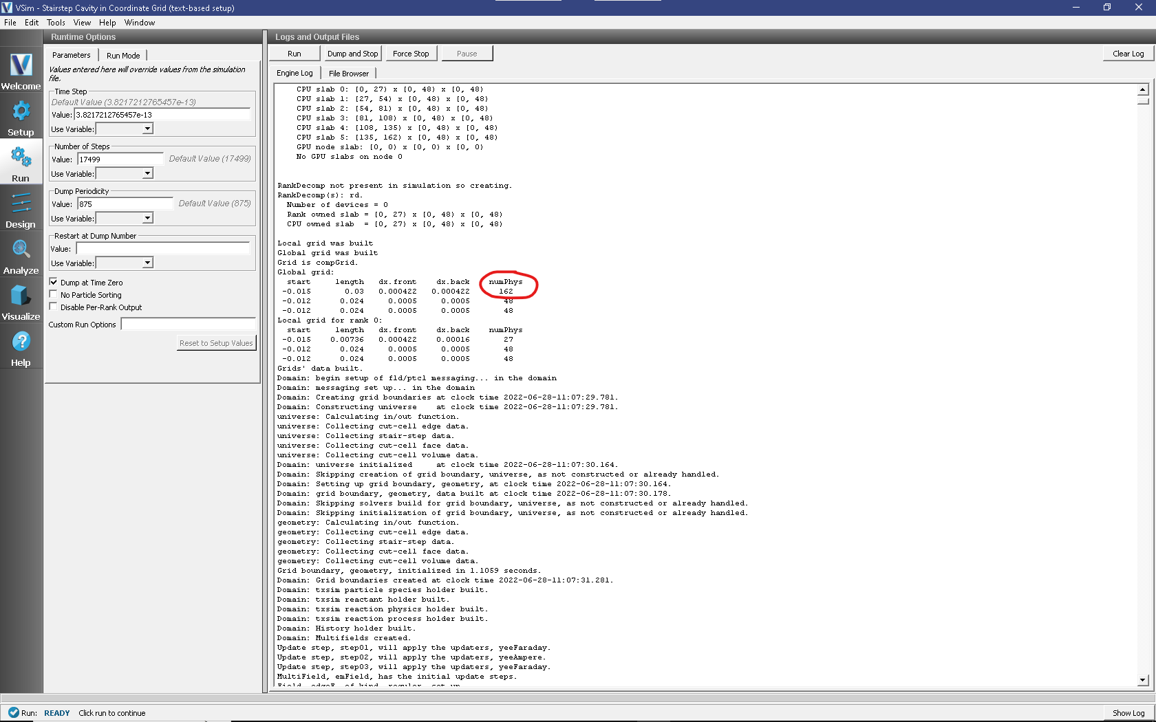
Fig. 391 Location of the numPhys output to be entered into the NX field by the user.
The simulation is now ready to run. Return to the Run Window, enter the desired values for Number of Steps and Dump Periodicity and click Run once again. The run has completed when you see the output, “Engine completed successfully” as shown in Fig. 392. This will require approximately two hours of computation time when run in parallel on four processors on a modern CPU.
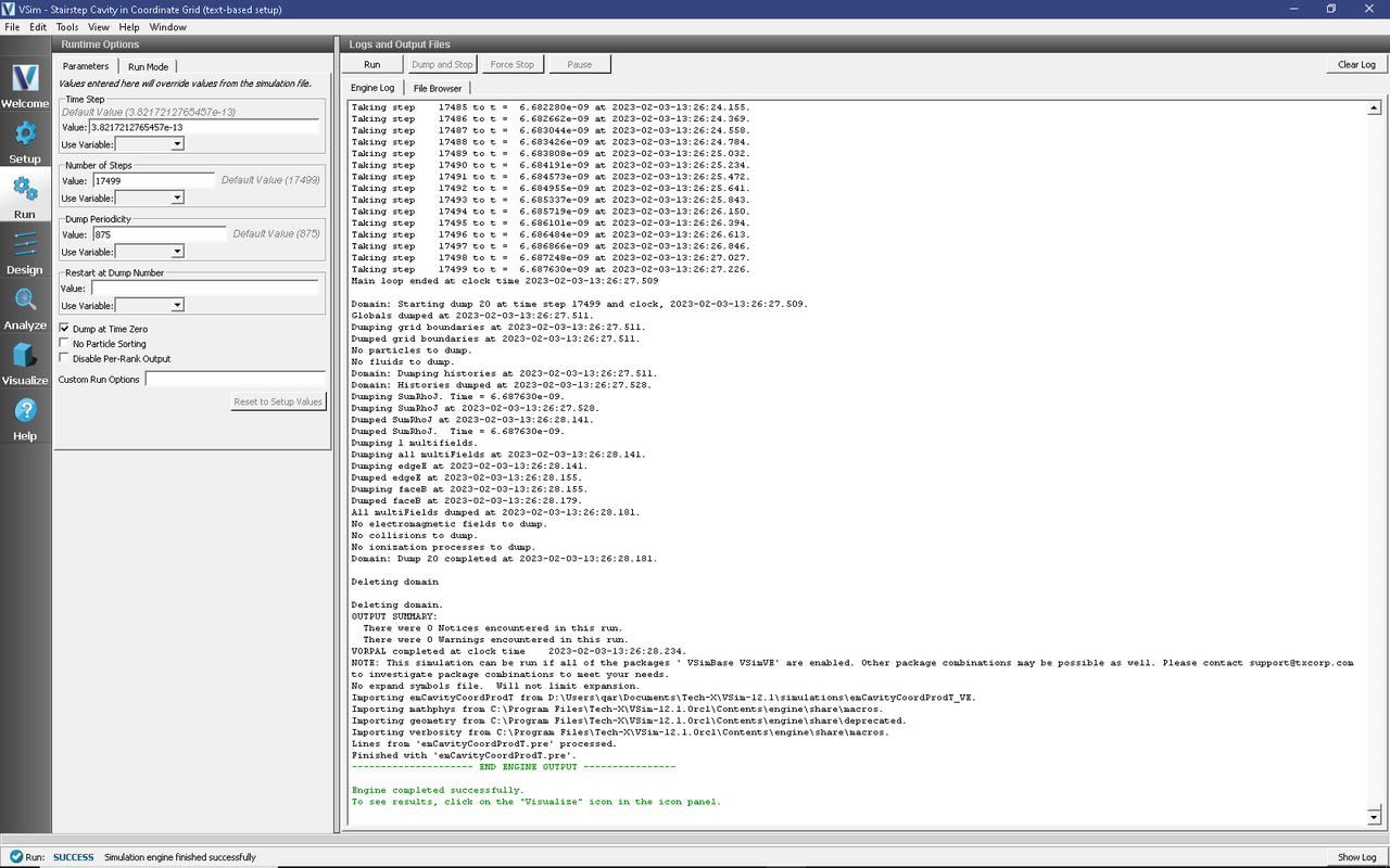
Fig. 392 The Run Window during the execution.
Visualizing the results
After performing the above actions, continue as follows:
Proceed to the Visualize Window by clicking Visualize in the left column of buttons.
To create the plot as shown in Fig. 393:
In the Variables section of the Visualization Controls pane, Expand Geometries
Select poly_surface
Check the Clip Plot box
Expand Meshes
Expand compGridGlobal
Select any of the grid choices, for they are all identical for this simulation
Check the Clip Plot box
Expand Scalar Data
Expand edgeE
Select edgeE_x
Check the Clip Plot box
Decrease the Opacity by moving the Opacity slider the left to better see the fields through the grid
At the bottom of the Visualization Results pane, move dump slider forward in time
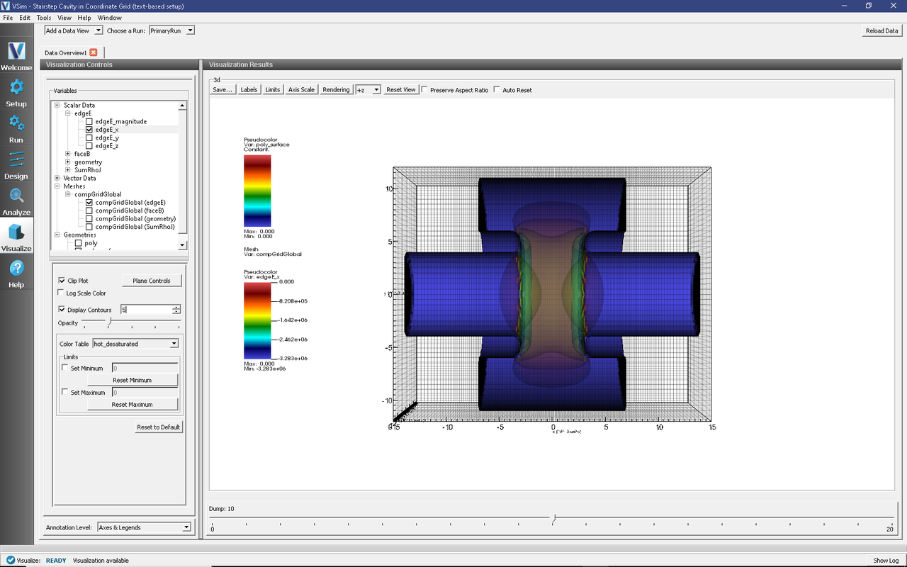
Fig. 393 Visualization of the \(x\)-component of the electric field in the simulation of a klystron cavity with a non-uniform mesh.
Further Experiments
The coordinateGrid system is also capable of creating non-uniform grids in cylindrical coordinates, by setting coordinateSystem = Cylindrical in the Grid block. The curlUpdaterCoordProd updater also works with the same settings in cylindrical coordinates.