A6 Magnetron 1: Modes (a6Magnetron1Modes.sdf)
Keywords:
- magnetron, cavity modes, A6
Problem Description
This VSimVE example simulates MIT’s cylindrical A6 magnetron cavity with no outlets in three dimensions. The structure is generated using shape primitives within the VSim composer. The cavity is excited by a sinc pulse ping using a distributed current source within one of the resonant cavities. The spectrum of the cavity is used to find the modes, and FDM is used to extract the exact mode profile of the cold cavity.
This simulation can be performed with a VSimVE license.
Opening the Simulation
The A6 Magnetron example is accessed from within VSimComposer by the following actions:
Select the New → From Example… menu item in the File menu.
In the resulting Examples window expand the VSim for Microwave Devices option.
Expand the Radiation Generation option.
Select “A6 Magnetron 1:Modes” and press the Choose button.
In the resulting dialog, create a New Folder if desired, and press the Save button to create a copy of this example.
All of the properties and values that create the simulation are
now available in the setup window as shown in
Fig. 399. You can expand the tree
elements and navigate through the various properties, making any
changes you desire. The right pane shows a 3D view of the
geometry, if any, as well as the grid, if actively shown. To
show or hide the grid, expand the Grid element and select or
deselect the box next to Grid.
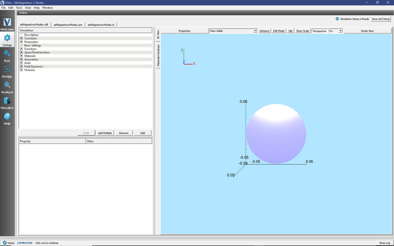
Fig. 399 Setup window for the A6 Magnetron example showing cathode and anode vanes only.
Simulation Properties
The A6 Magnetron example includes several constants for easy adjustment of simulation properties. User changeable parameters include:
RADIUS_ANODE → Inner radius of anode.
RADIUS_ANODE_OUTER → Outer radius of anode.
ANGLE_CAVITY → Angle of resonant cavity openings, in degrees.
THICKNESS_WALL_OUTER → Thickness of all walls.
WIDTH_VANES → Total width of anode vanes in z-direction.
RADIUS_CATHODE → Radius of the emitting section of the cathode.
RADIUS_CATHODE_INNER → Radius of the inner section of the cathode.
WIDTH_CATHODE → Width (in z-direction) of the emitting section of the cathode.
FREQ_LOW → Lower frequency of excitation source range.
FREQ_HIGH → Upper frequency of excitation source range.
(X,Y,Z)POS_CURR → Position of excitation distributed current source.
(XY,Z)SIZE_CURR → Size of excitation distributed current source region.
(X,Y,Z)POS_HIST → Position of electric field history.
The axis of the cavity coincides with the z-axis and the center is at z = 0. The emitting cathode region is 4.0 cm long. All surfaces are perfect electric conductors. Histories of the electric and magnetic fields are taken at the inside of one of the cavities to find the modes. The FFT of the history shows the mode frequencies, and the exact value and profile is found using extractModes.py - Extract Modes Analysis Scripts.
The excitation frequency range can be set using the constants FREQ_LOW and FREQ_HIGH. The total excitation time is calculated in TIME_EXCITE. The simulation should be run for longer than TIME_EXCITE to allow the excitation source to complete.
Running the Simulation
After performing the above actions, continue as follows:
Proceed to the run window by pressing the Run button in the left column of buttons.
To run the file, click on the Run button in the upper left corner of the right panel. You will see the output of the run in the right pane. The run has completed when you see the output, “Engine completed successfully.” This is shown in Fig. 400.
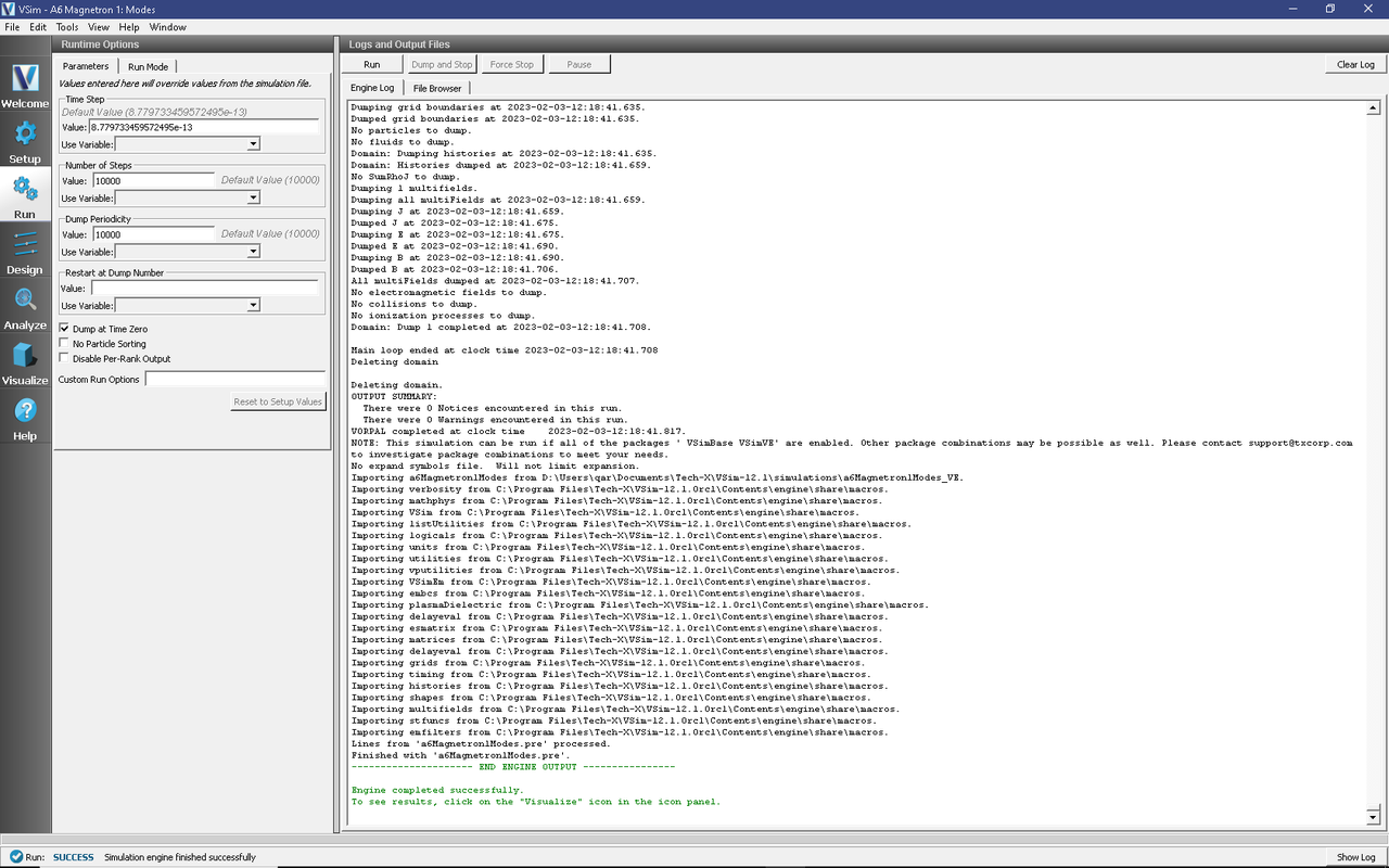
Fig. 400 Run window for the A6 Magnetron mode extraction example after the initial run..
The simulation is best run in two steps: The first with course dump periodicity to excite the modes, and the second with fine dump periodicity to observe the modes.
Initially, the simulation is run for 10,000 time steps, writing one dump file at the end, to allow the current source excitation to finish.
After the initial run, change the Number of Time Steps to 2,000, the Dump Periodicity to 50, and enter 1 into Restart at Dump Number. This will record details of the excited field after the source has finished.
Visualizing the results
After performing the above actions, continue as follows:
Proceed to the Visualize window by pressing the Visualize button in the left column of buttons.
To visualize a run to determine the resonant frequency, select History from the Data View pull-down menu. Select outE_0 for Graph 1 and Graph 2, and click Fourier Amplitudes (dB) to the left of one of the outE_0 plot in the Visualization Results pane. .
Proceed to the Visualize window by pressing the Visualize icon in the left panel.
Select History under Data View.
Then for Graph 2 select the Fourier Amplitudes (dB) checkbox * In the upper right corner of the same plot, select Limits and set X-Axis max to 1e10.
The result should be that shown in Fig. 401.
Note that running the simulation longer will more sharply resolve the mode frequencies in the FFT.
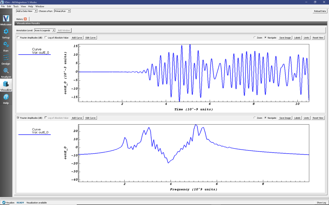
Fig. 401 Fourier transform of outE_0 versus time (in Hertz).
Analyzing the Results
It is possible to extract the modes of the A6 magnetron cavity via post processing using the extractModes.py - Extract Modes Analysis Script as follows:
Press the Analyze button in the left column of buttons.
Select extractModes.py(default).
Enter the following parameters in the appropriate fields:
simulationName = a6Magnetron1Modes
field = B
beginDump = 2
endDump = 41
nModes = 7
numberUniformPts = 20
numberRandomPts = 100
randomSample = unchecked
construct = checked
Click the Analyze button in the upper right corner of the window.
Three columns of data with the titles “freq [Hz]” (Eigenmode frequency), “invQ” (inverse quality factor), and “SVD” (singular value decomposition) will be output in the right pane. The analysis has completed when you see the output “Analysis completed successfully.” One can see 7 modes in Fig. 402.
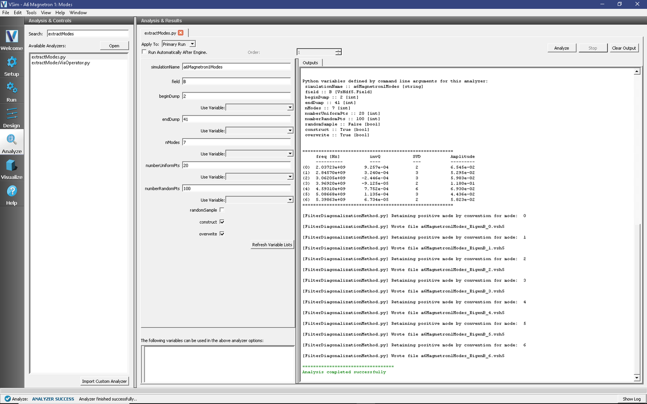
Fig. 402 The Analysis Window, showing 7 modes.
Proceed to the Visualize window by pressing the Visualize icon in the left panel.
Click the ‘Reload Data’ button in the top-right corner.
Select Data Overview under Data View.
Expand Scalar Data
Expand B
Select B_z (EigenB).
Select the Clip Plot checkbox.
Move the dump slider first to dump 2 and then to dump 5.
The axial magnetic field inside the cavity during the \(\pi\) and \(2\pi\) mode operations are shown in Fig. 403 and Fig. 404, respectively:
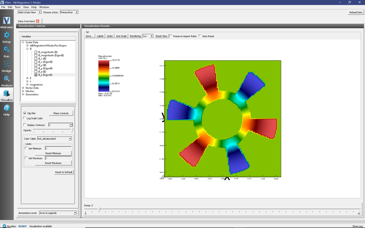
Fig. 403 Visualization of the axial B-field in the \(\pi\) Eigenmode.
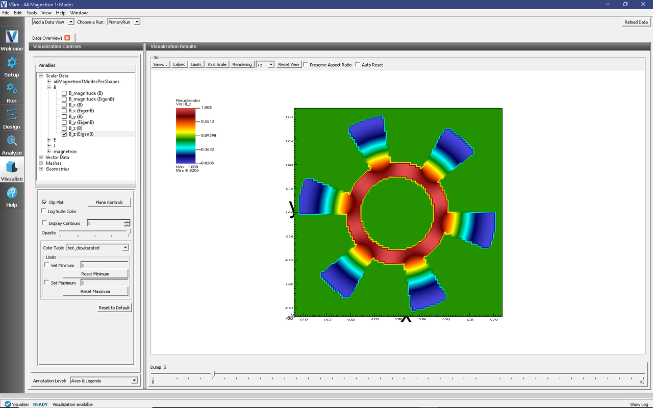
Fig. 404 Visualization of the axial B-field in the \(2\pi\) Eigenmode.
Further Experiments
The values of FREQ_LOW and FREQ_HIGH can be adjusted to find additional modes, or to focus in on a specific mode. Narrowing the excitation range to fewer modes will produce a mode-accurate frequency and Q-factor extraction for the mode.