Klystron (klystron.sdf)
Keywords:
- klystron
Problem description
This VSimVE example simulates a two cavity klystron in three dimensions. The first cavity is driven at its lowest resonant frequency. The resultant cavity voltage creates a velocity modulation in the electron beam which translates to charge modulation as the beam travels in the tube between cavities. The charge modulation then drives the second cavity. The cavities are loaded to give them finite Q.
This simulation can be performed with a VSimVE or VSimPD license.
Opening the Simulation
The Klystron example is accessed from within VSimComposer by the following actions:
Select the New → From Example… menu item in the File menu.
In the resulting Examples window expand the VSim for Microwave Devices option.
Expand the Radiation Generation option.
Select Klystron and press the Choose button.
In the resulting dialog, create a New Folder if desired, and press the Save button to create a copy of this example.
All of the properties and values that create the simulation are now available in the setup window as shown in Fig. 438. You can expand the tree elements and navigate through the various properties, making any changes you desire. The right pane shows a 3D view of the geometry, if any, as well as the grid, if actively shown. To show or hide the grid, expand the Grid element and select or deselect the box next to Grid.
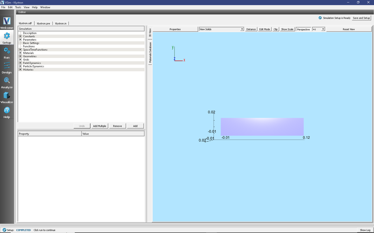
Fig. 438 Setup Window for the Klystron example.
This example illustrates two methods for generating geometries. Under Geometries in the elements tree there are two paths, CSG and load1Geom. The CSG components are constructed from primitives within VSim. The load1Geom was imported as an STL file. Highlighting any geometry under the CSG group shows how it was created, either as a primitive with parameters or by operations on other shapes.
Simulation Properties
This simulation is set up to do a Power Run with full capabilities. After completing the Power Run and visualizing the results, you may wish to refine the performance of the klystron by adjusting the setup. Some useful tuning procedures are described in the Further Experiments section. These include the Resonant Frequency Run and the Attenuation Calibration Run.
Some constants that you may wish to modify include:
FREQUENCY:The frequency (in Hz) at which the signal across cavity is driven. This can be tuned to the resonant frequency once determined.
BEAMRADIUS: The radius of the emitted beam of electrons into the klystron.
BEAMCURRENT: The current of the electron beam.
Running the Simulation
With the default setup, complete the Power Run with the following steps:
Proceed to the Run window by pressing the Run button in the left column.
To run the file, click on the Run button in the upper left corner of the right pane. You will see the output of the run in the right pane. The run has completed when you see the output, “Engine completed successfully.” This is shown in Fig. 439 below.
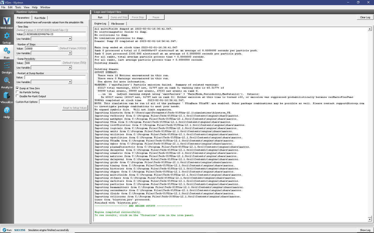
Fig. 439 The Run Window at the end of execution.
Visualizing the Results
After the simulation run has completed successfully, you may proceed to the Visualize Window by pressing the Visualize button in the left column. To reproduce Fig. 440 follow these steps:
Select Data Overview from the Data View pull-down menu.
Expand Particle Data
Expand electrons0
Select electrons0_ux
Expand Geometries
Select poly (klystronPecShapes)
Select the Clip Plot checkbox
Step through time using the dump slider on the bottom of the right pane.
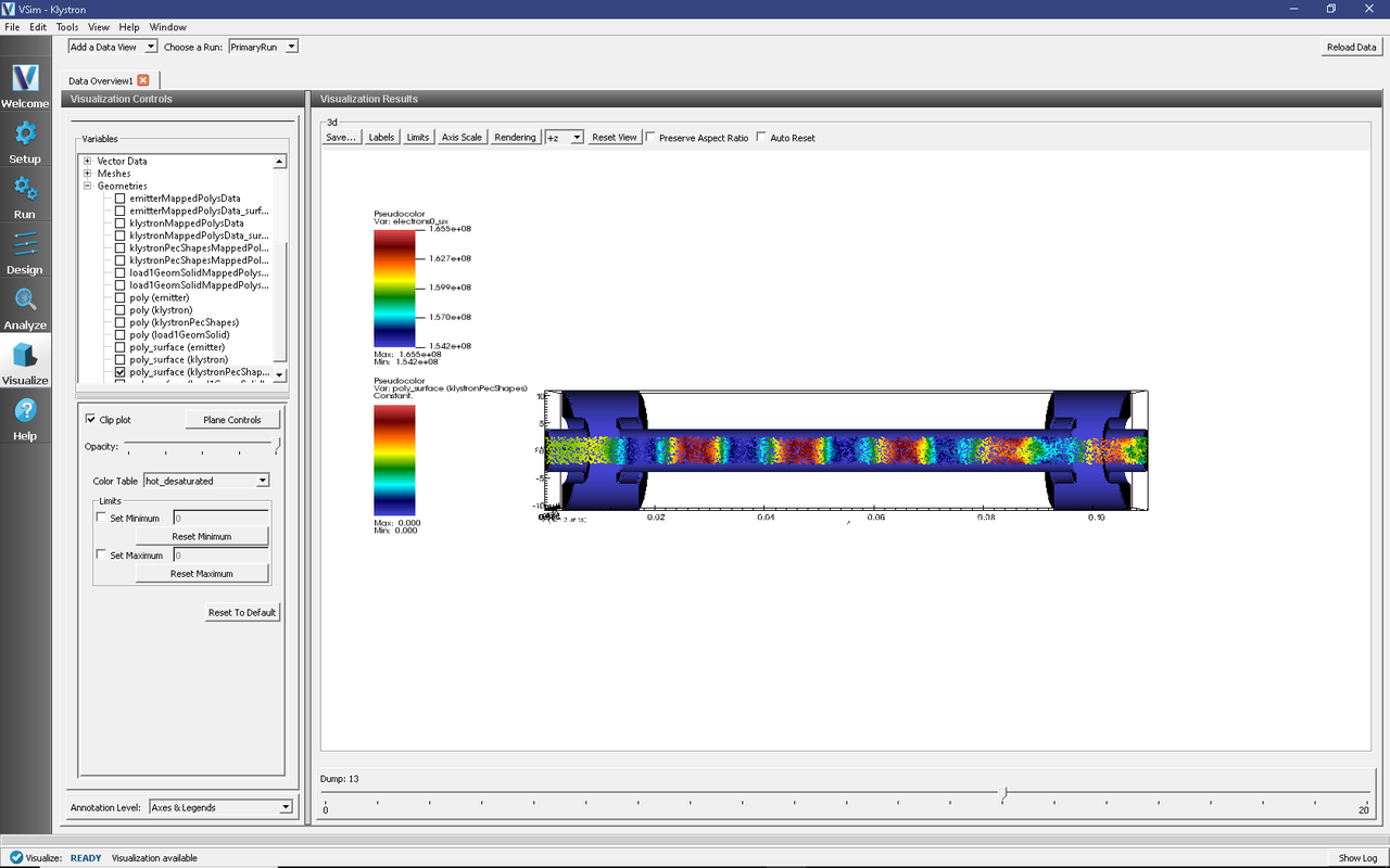
Fig. 440 A power run with an electron beam.
Further Experiments
The Attenuation Calibration Run and Resonant Frequency Run are outlined below. These experiments will allow you to tune the klystron. You may want to iterate through these experiments to get the desired performance. Once the cavity performance is satisfactory you can repeat the Power Run to see the effects on the electrons. To see the full behavior of the device, increase the number of steps to (5 x Default). This will allow you to see the saturation of the second cavity.
Resonant Frequency Run
To determine the resonant frequency of the first cavity we will analyze the fourier transform of its voltage. In the Setup window, under Basic Settings, set particles to no particles. Then, under SpaceTimeFunctions, in ring1J change the turn on function to from “standard” to “up and down”. This will ping Cavity 1 and allow us to observe the ringing signal. Run the simulation with this setup.
To determine the resonant frequency proceed to the Visualize window. Select History from the Data View pull-down menu. Click FFT to the left of the Cavity1Voltage plot in the Visualization Results pane. The resulting plot will resemble Fig. 441. Zoom in on the maximum of this plot to determine the resonant frequency. You can now update the FREQUENCY under Constants in the Setup window with this new value and use it to drive future simulations.
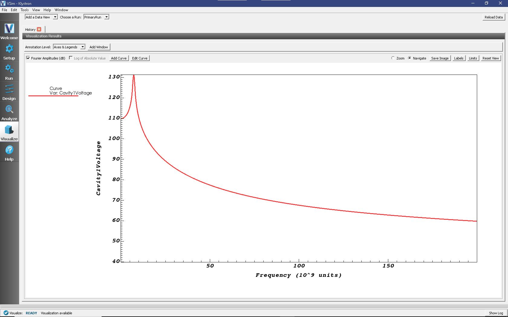
Fig. 441 Fourier transform of Cavity1_Voltage versus time (0-2 GHz).
Attenuation Calibration Run
The user can integrate this run type in order to calibrate the observed attenuation to the desired loss. The attenuation can be tuned by modifying the conductivity of the material, resistive damper. The Q of the cavity can be computed using a feature of the Analysis Tab, as described below.
For the Attenuation Calibration Run, use the same Setup as the Resonant Frequency Run. After running the simulation, the quality factors, \(Q_1\) and \(Q_2\), for cavities 1 and 2 can be calculated using the computeInverseQ.py script in the Analyze window.
Press the Analyze button in the left column of buttons.
Select the computeInverseQ.py analyzer, then Open.
Enter Cavity1Voltage or Cavity2Voltage in the historyName field to designate the history to analyze.
Enter the value of the FREQUENCY constant as defined in the Setup window in the frequency field to designate the frequency at which the history will be analyzed.
Update the outputFileName field if desired
Click the Analyze button in the top right corner of the window. As shown in Fig. 442 below. Two columns of data with the titles “Time (s)” and “Inverse Q” will be output in the right pane. The analysis has completed when you see the output “Analysis completed successfully.”
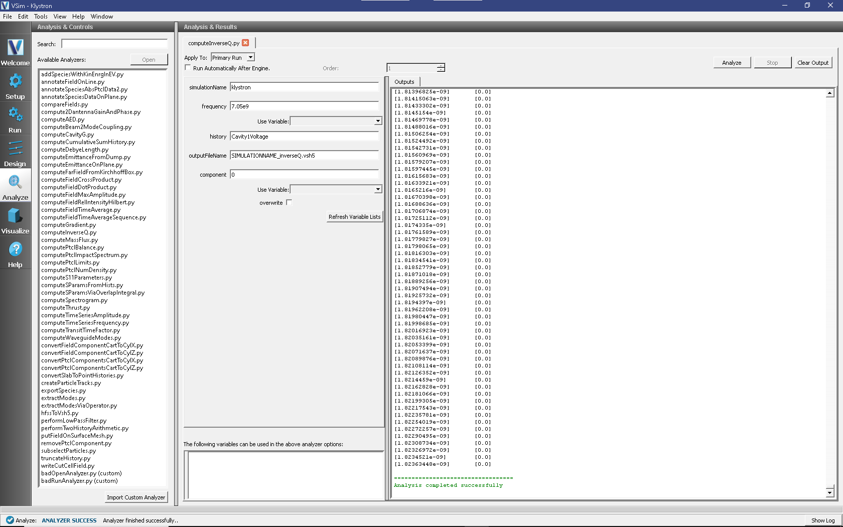
Fig. 442 The Analysis window at the end of execution of the computeInverseQ.py script.
Scrolling through or plotting the output data in the Visualize window enables the user to understand the Klystron’s performance. The user may iterate this run type to achieve the desired attenuation.