Helix Traveling Wave Tube 2: Impedance and Attenuation (helixTwt2ImpedAtten.sdf)
Keywords:
- Helix TWT Impedance and Attenuation Run
Problem description
This VSimVE example is one of a set of simulations showing different calculations to aid the design of a helix traveling wave tube (TWT) in three dimensions. The 100-turn helix with end feeds is imported from a CAD file, but all other geometrical parts are created with the Constructive Solid Geometry (CSG) capabilities within VSimComposer.
An input signal is sent into a short section of coaxial input waveguide and a similar section of coaxial waveguide at the opposite end of the tube provides an output power port. The geometry includes three dielectric support rods, each clad by a section of resistive tubing for attenuation. The Impedance and Attenuation simulation enables the user to calculate the transverse impedance and Pierce interaction impedance of the helix TWT. The transverse impedance is relevant for impedance matching at the input and output coaxial ports, and the Pierce interaction impedance is related to the interaction of the particles with the signal, and thus the signal gain.
The user may wish to run this simulation type multiple times, varying parameters such as the coax radius and dielectric permittivity, in order to result in a design with the correct impedance parameters.
Related simulations:
Helix Traveling Wave Tube 1: Dispersion (helixTwt1Dispersion.sdf)
Helix Traveling Wave Tube 3: Power Run (helixTwt3PowerRun.sdf)
This simulation can be performed with a VSimVE or VSimPD license.
Opening the Simulation
The Helix TWT Impedance and Attenuation example is accessed from within VSimComposer by the following actions:
Select the New → From Example… menu item in the File menu.
In the resulting Examples window expand the VSim for Vacuum Electronics option.
Expand the Radiation Generation option.
Select “Helix Traveling Wave Tube 2: Impedance and Attenuation” and press the Choose button.
In the resulting dialog, create a New Folder if desired, and press the Save button to create a copy of this example.
All of the properties and values that create the simulation are available in the Setup Window as shown in Fig. 423, with the Elements Tree in the upper center, and the Property Editor in the lower center. The right pane shows a 3D view of the geometry as well as the grid, if its visibility has been activated (which it was not when this image was captured).
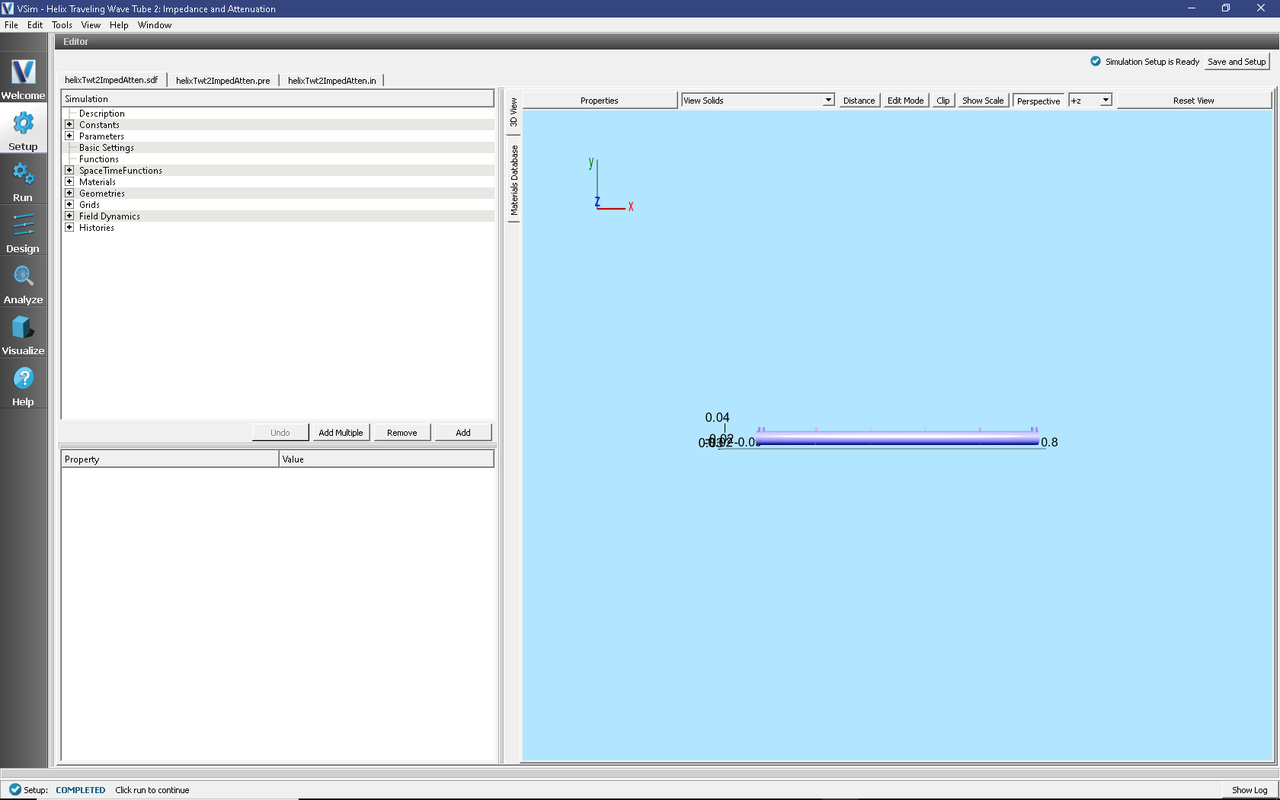
Fig. 423 Setup Window for the Helix TWT impedance and attenuation example.
Geometry details
The various geometrical objects can all be seen in the tree by pulling down the bar separating the Elements Tree from the Property Editor and then expanding Geometries, CSG, and Grids. Make sure tube and Grid are unclicked, helixWithFeedsGeom is clicked, and that the Toggle Axes button is set to remove the axes from the view. This allows one to see the interior geometrical objects, including the incoming feed, the dielectric support rods, the resistive tubes in the center, the particle emission disk at the left, and various planes where measurements are taken.
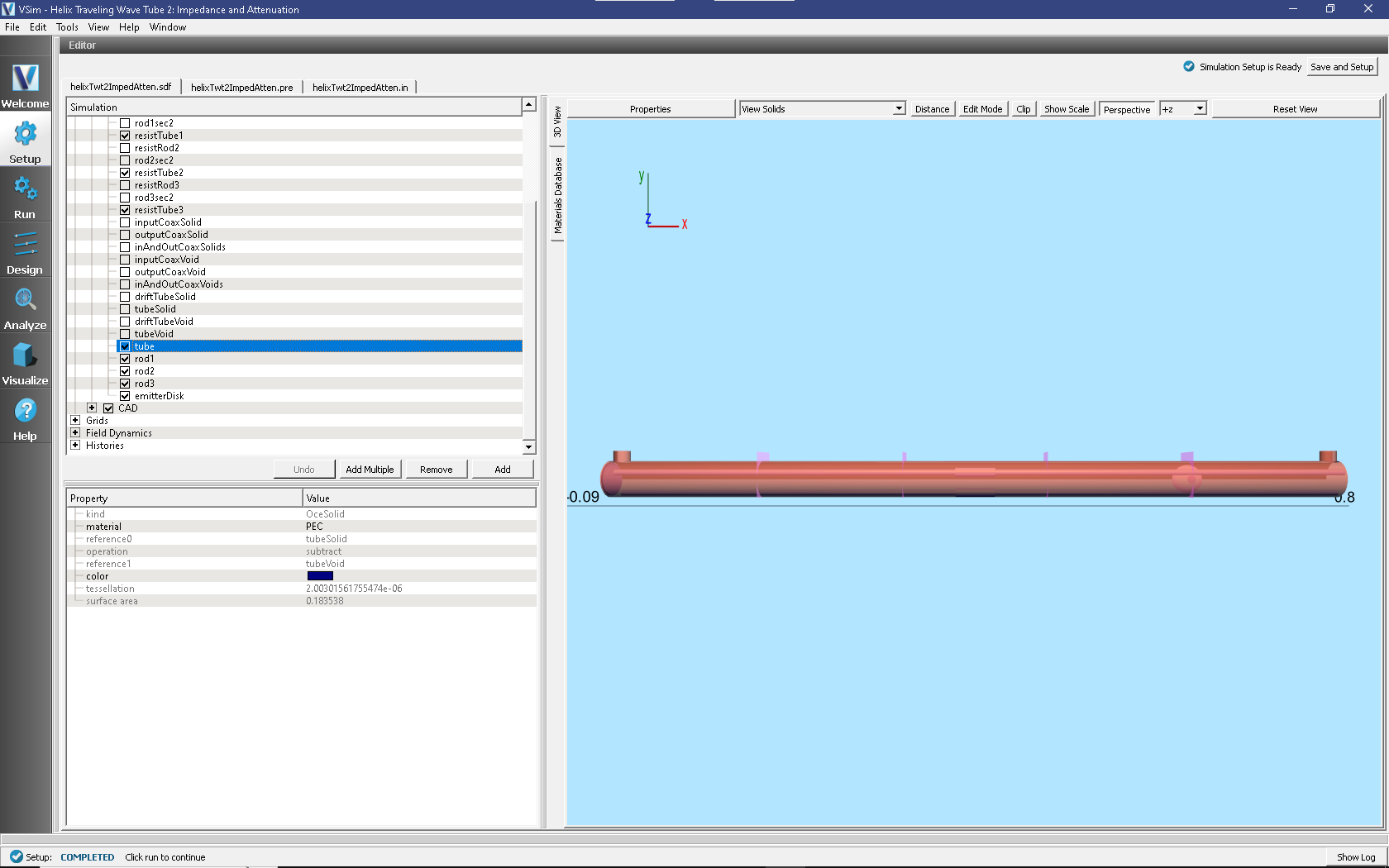
Fig. 424 Interior geometry for the Helix TWT impedance and attenuation example.
Constants and Parameters
Pulling the separator bar between the Elements Tree and the Property Editor and opening the Constants part of the tree gives the view shown in Fig. 425.
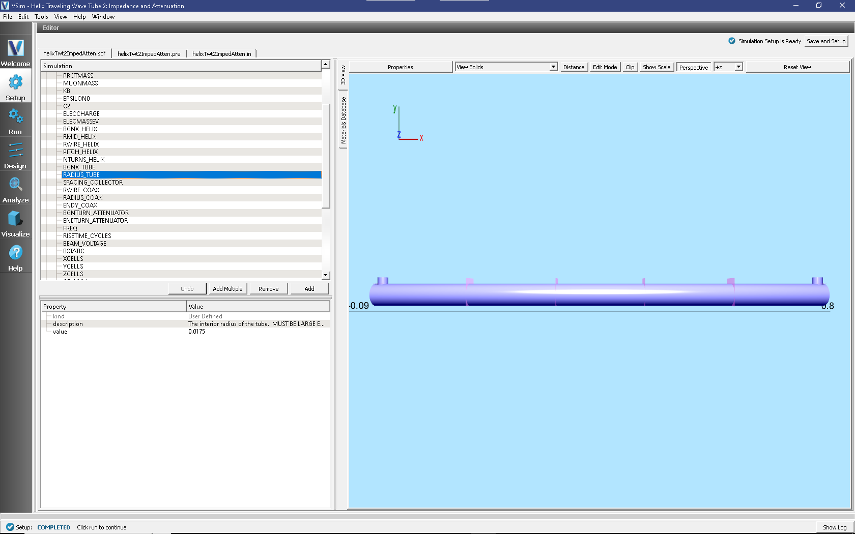
Fig. 425 Constants for the Helix TWT impedance and attenuation example.
There are three types of constants. The first set of constants,
from PI through ELECMASSEV are not changeable by
the user. These are the various mathematical and physical
constants that the simulation will use. The second set of
constants are those with HELIX in the name. These must
correspond to the helix geometry, the beginning, mid-radius, wire
radius, pitch, and number of turns of the helix. These cannot be
set arbitrarily, as the helix was imported as an STL file.
Instead they must be set to match the imported helix parameters.
The remaining constants define fundamental geometry quantities,
such as where the tube begins and its radius, other physical
simulation parameters, such as the wave frequency, and numerical
parameters, such as the number of cells in each direction.
Moving the scroll bar and opening the Parameters part of the tree shows the Parameters, values that come from arithmetically combining constants and other parameters. This is shown in Fig. 426.
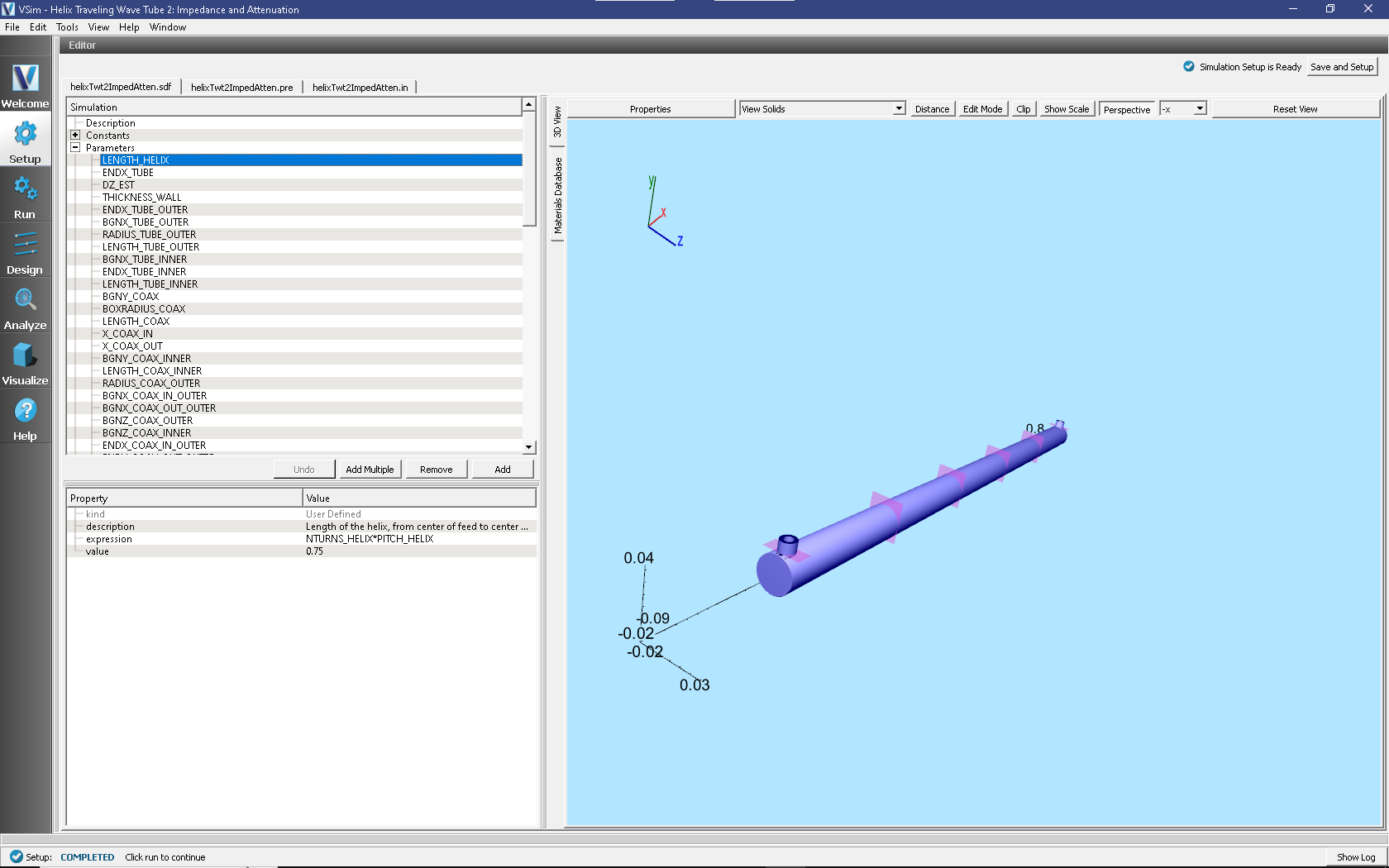
Fig. 426 Parameters for the Helix TWT impedance and attenuation example.
As an example, LENGTH_HELIX is shown. The expression
shows that this is the number of helix turns times the helix
pitch. It also shows the value. Of course, the expression is
editable, while the value is not.
Both constants and parameters have a description field that allows the user to document the quantity.
Materials
To bring materials in the simulation, in the right pane, select the Database tab, select one or more materials (with ctrl-click) and hit the button Add To Simulation. The materials will then appear under Materials in the tree view. At this point one can change the properties of the materials including the name. In this example we imported resistive damper, changed its name to LossyMaterial, and changed its value of conductivity to 0.55. This is shown in Fig. 427.
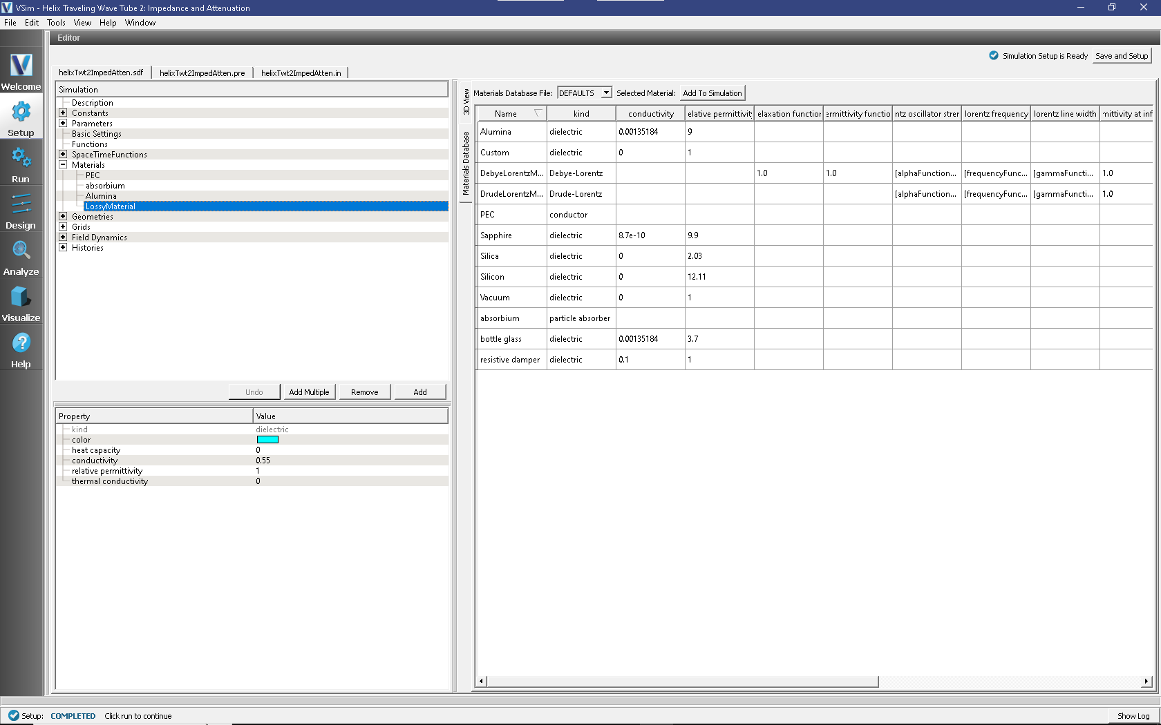
Fig. 427 Materials for the Helix TWT impedance and attenuation example.
Once one has materials in the simulation, one can set the materials of any of the geometries. Click on the geometry, then in the Property Editor pane, double click on the material value. A context menu will allow you to set the material of the geometry to any material in the simulation.
Running the simulation
After performing the above actions, continue as follows:
Proceed to the run window by pressing the Run button in the left column of buttons.
To run the file, click on the Run button in the upper left corner of the right panel. You will see the output of the run in the right pane. The run has completed when you see the output, “Engine completed successfully.” This is shown in Fig. 428.
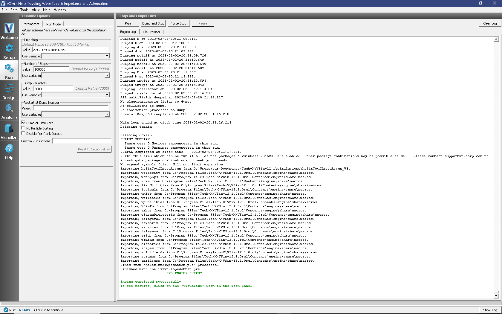
Fig. 428 The Run Window at the end of execution.
The simulation to determine the impedance should run long for any mismatch at the outgoing boundary to stabilize. That is, the simulation must be run long enough for the electromagnetic wave to reach the far end of the tube and for any reflections to return some distance to the last history in the tube. This will take about 100,000 steps. On a 4-core machine, we have observed 0.23s/step, so this simulation will take about 7 hours. This simulation parallelizes well up to 16 cores, so with a sufficient license and workstation or cluster, one can bring this simulation time down to about 2 hours.
Visualizing the results
After performing the above actions, continue as follows:
Proceed to the Visualize Window by pressing the Visualize button in the left column of buttons.
To see the fields inside the tube as shown in Fig. 429, continue as follows:
Select Data View: Data Overview
Expand Scalar Data then D, then select field D_y.
Check the Clip Plot box, which cuts through the data at the \(z=0\) plane.
Check Set Minimum and set it to -400, then check Set Maximum, set it to 400.
Expand Geometries then select poly (rod1).
Check the Clip Plot box
Move the dump slider forward in time to see the evolution.
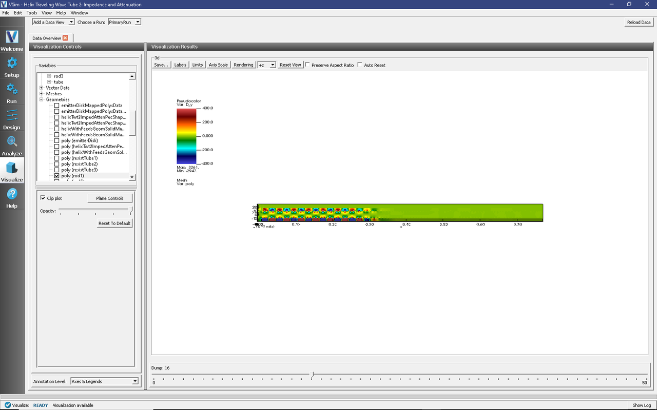
Fig. 429 The transverse displacement field, Dy, on the central x-y plane at dump 31.
This plot shows the transverse displacement field. Once can see that it is confined inside the tube (sanity check), and that it is most intense inside the dielectric rod at the bottom. The field is larger at the left, as it is just entering and propagating down the tube.
At any time one can leave this visualization pane to move back to the run pane to see how the simulation is progressing.
The longitudinal field inside the tube is shown in Fig. 430, which can be obtained by the steps:
Select Data View: Field Analysis
Select Field E_x.
Select Horizontal under Lineout Settings, set the Intercept to
0, and click Perform Lineout.Under Layout select Stacked 2d/1d
Move the dump slider forward in time to see the evolution.
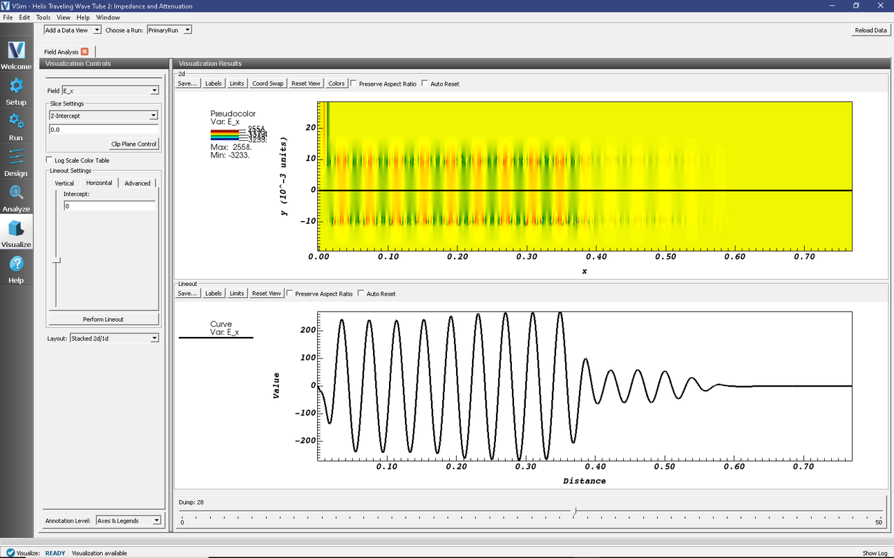
Fig. 430 The longitudinal field, Ex, on axis at dump 28, which is time step 56,000.
As seen in Fig. 430, the
longitudinal field has dropped from about 240 V/m to
about 68 V/m in the center of the simulation where the
resistive tubes are. This corresponds to about 14 dB of
attenuation. The purpose of this attenuation is to have
sufficient damping so that reflections coming back from the end
to the beginning and then reflection again do not grow, as that
would change the device into an oscillator, with energy growth
that could destroy the system. If the Helix Traveling Wave Tube 3: Power Run (helixTwt3PowerRun.sdf)
shows that this is happening, one can return to this run and
increase the conductivity of the LossyMaterial or the length of
the resistive tube (through BGNTURN_ATTENUATOR and
ENDTURN_ATTENUATOR) to provide more attenuation.
Histories contain the time evolution of quantities defined in the input file. These can be seen by selecting the Data View, History. To determine various impedances we want particular histories obtained by the process:
Select Data View: History
Under Graph 1 select poyntingA
Under Graph 2 select transverseVoltageA
Under Graph 3 select EonAxisA_0
Under Graph 4 select <None>
The result is shown in Fig. 431. The power through the plane was defined such that incoming is negative.
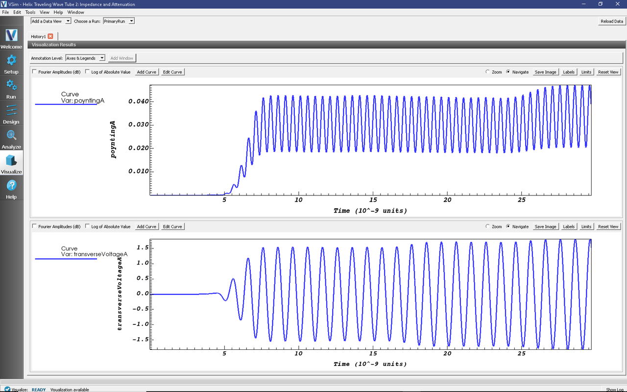
Fig. 431 Poynting power (W), transverse voltage (V), and electric field (V/m), at Plane A, along the helix TWT as a function of time (s).
Impedance parameters of interest are the transverse impedance
and the Pierce interaction impedance
where \(P\) is the poynting power (recorded in the history poyntingA), \(V_t\) is the transverse Voltage amplitude (recorded in the histories transverseVoltage), \(E_x\) is the electric field amplitude (recorded in the history EonAxis), and \(\lambda\) is the wavelength of the field along the helix TWT axis.
The histories show the graphs of these quantities. To get precise values for any of these, one can press the Limits button, which will pop up a window with the precise values. First, the X-Axis limits show that the units are \(ns\). Secondly, one needs to choose a consistent time period, where all amplitudes are roughly constants. The period \(28ns < t < 32ns\) is chosen. One can now adjust the limits until the peaks line up with the limits. We want average poynting power. We find \(P_{min} = 18. \ mW\) and \(P_{max} = 44. \ mW\). Hence, \(P_{av} = 31. \ mW\). During that same time interval we find \(V_t = 2.4 \ V\) and \(E_x = 240 \ V/m\).
Fig. 430 can be used to obtain the wavelength. One can see four wavelengths between \(0.20m\) and \(0.357m\). Therefore the wavelength is \((.357m-.20m)/4 = 0.039m\)
We now compute
and the Pierce interaction impedance is
Further Experiments
As noted above, one can change the attenuation by varying the conductivity of the resistive tubs or their length. For any given length, there is a maximum attainable attenuation, as there is no attenuation at zero conductivity (infinite resistance, i.e., vacuum) and none as well at infinite conductivity (metallic shielding). So if more than 14 dB attenuation is needed one can vary the conductivity, but a maximum will be observed, and if that is insufficient one will have to vary the rod length.
With additional computing resources, one could increase the grid resolution so that the resistive tube could be made thinner. As it is made thinner, one can go to greater conductivity without having the skin depth less than the resistive tube thickness.
The coupling is determined by the transverse impedance of the structure, which in turn depends on the capacitance provided by the rods. Varying the relative permittivity changes the transverse impedance.