Helix Traveling Wave Tube 3: Power Run (helixTwt3PowerRun.sdf)

Keywords:

Helix TWT Power Run

Problem description

This VSimVE example is the last of a set of simulations showing different calculations to aid the design of a helix traveling wave tube (TWT) in three dimensions. The 100-turn helix with end feeds is imported from a CAD file, but all other geometrical parts are created with the Constructive Solid Geometry (CSG) capabilities within VSimComposer.

An input signal is sent into a short section of coaxial input waveguide and a similar section of coaxial waveguide provides an output power port. The geometries in and constant parameters of this simulation are described in more detail in Helix Traveling Wave Tube 2: Impedance and Attenuation (helixTwt2ImpedAtten.sdf). Electrons are injected at the left end of the tube. Gain can be computed from the ratio of voltages in the input and output waveguides.

The user may wish to run this simulation type multiple times, varying parameters such as the input signal power and the electron energy, in order to result in a design with maximum output power.

Related simulations:

This simulation can be performed with a VSimVE or VSimPD license.

Opening the Simulation

The Helix TWT Power Run example is accessed from within VSimComposer by the following actions:

Select the New → From Example… menu item in the File menu.
In the resulting Examples window expand the VSim for Vacuum Electronics option.
Expand the Radiation Generation option.
Select “Helix Traveling Wave Tube 3: Power Run” and press the Choose button.
In the resulting dialog, create a New Folder if desired, and press the Save button to create a copy of this example.

All of the properties and values that create the simulation are now available in the Setup Window as shown in Fig. 432. You can expand the tree elements and navigate through the various properties. Some of these changes will affect the geometry, and so one should review the look of the geometry in the right pane as one changed geometrical variables. To show or hide the grid, expand the Grid element and select or deselect the box next to Grid. One can, e.g., hide the tube to see inside it.

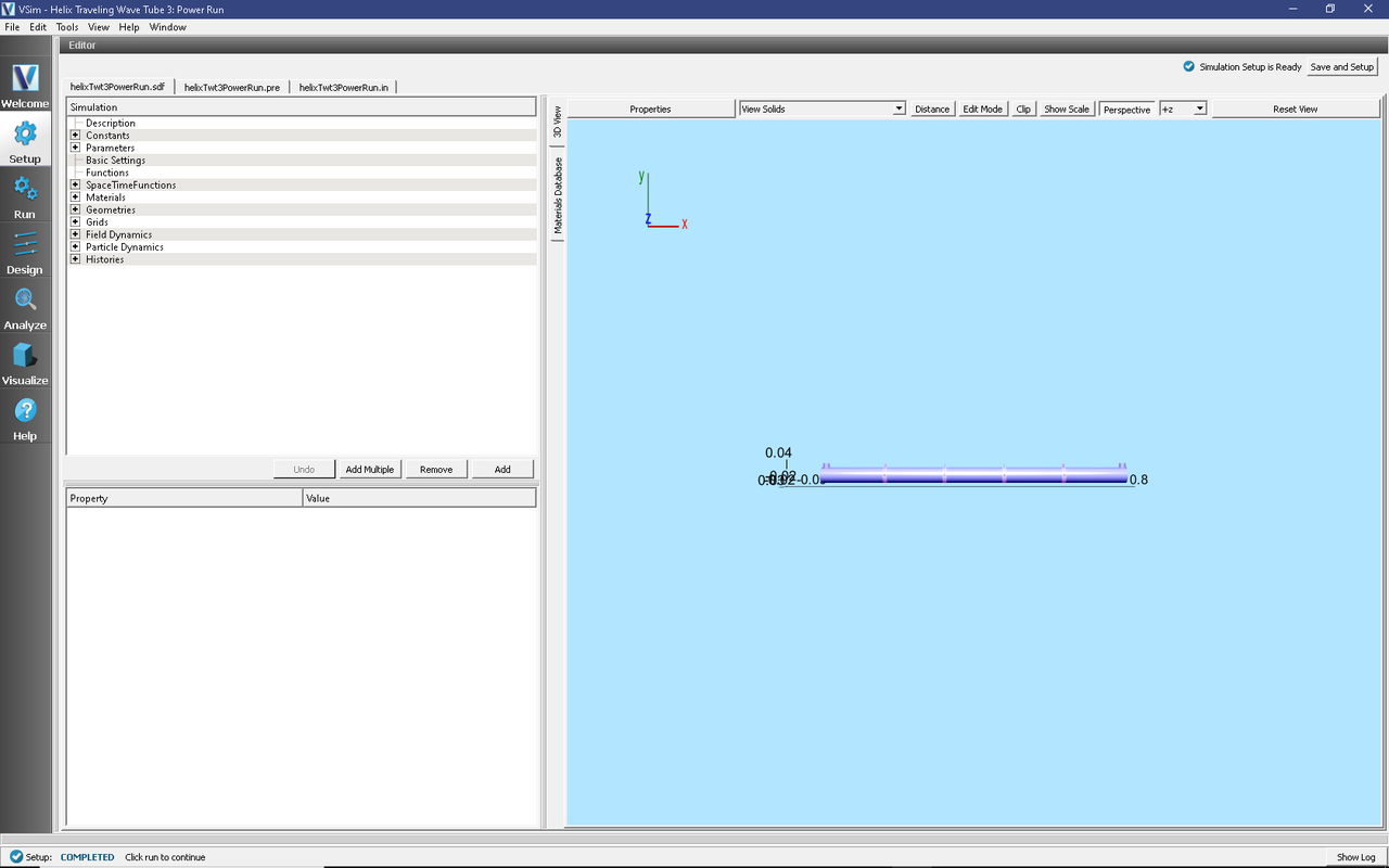
Fig. 432 Setup Window for the Helix TWT example.

The geometry of the helix can be made more visible by unselecting the tube and emitter disk parts under Geometries/CSG in the tree (e.g. driftTubeSolid, tubeSolid, driftTubeVoid, tubeVoid, tube, and emitterDisk) or by changing their color property and selecting a low alpha on Windows or Linux (or opacity on Mac). See color property setting in the User Guide.

Additional detail of the geometry is shown in figure Fig. 433. Fig. 432 shows the dielectric rods and Fig. 433 shows how the coaxial waveguide connects to the helical wire.

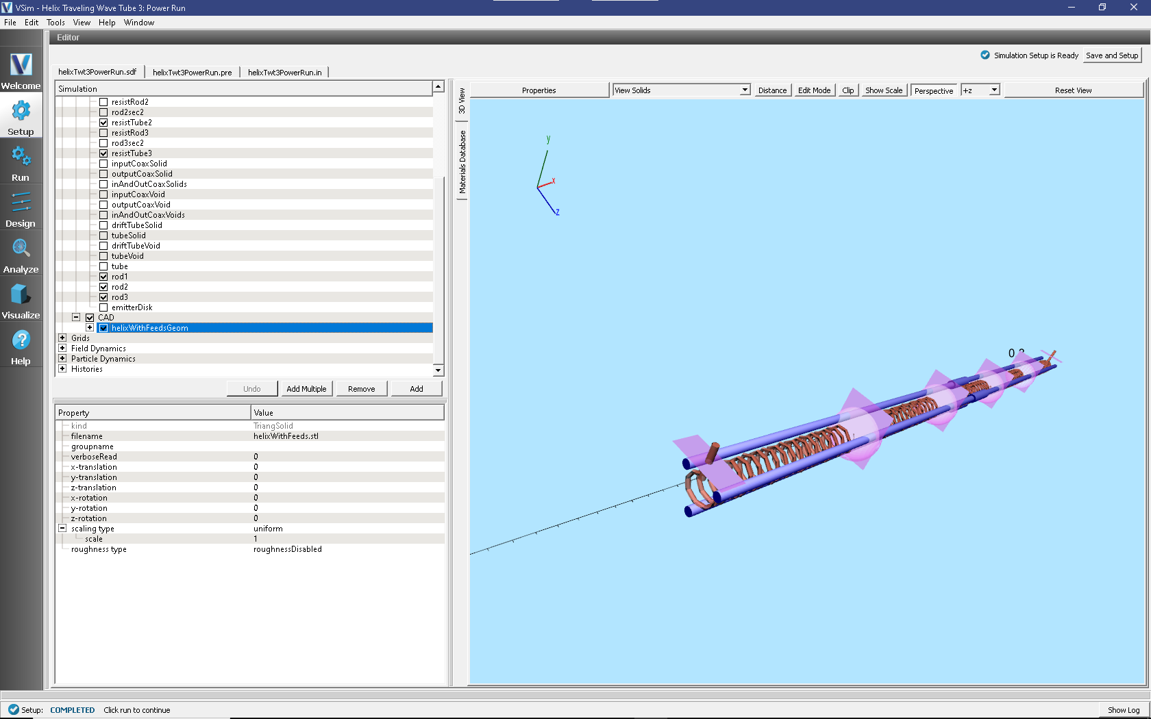
Fig. 433 A view in through the input coax.

Running the simulation

After performing the above actions, continue as follows:

Proceed to the run window by pressing the Run button in the left column of buttons.
To run the file, click on the Run button in the upper left corner of the right panel. You will see the output of the run in the right pane. The run has completed when you see the output, “Engine completed successfully.” This is shown in Fig. 434.

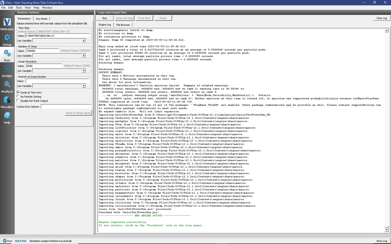
Fig. 434 The Run Window at the end of execution.

The default number of time steps will run the simulation long enough to verify that the electron beam is traveling down the tube, that the input signal has entering the simulation and propagated down the tube, that the amplified signal is leaving the system, and that the amplification has reached a steady state. However, the simulation has not been run long enough to ensure that there are no deleterious, backward wave oscillations. To determine that, one should run the simulation twice as long (ensuring a backward and forward traversal) or more, depending on the growth rate of the oscillation.

Visualizing the results

After performing the above actions, continue as follows:

Proceed to the Visualize Window by pressing the Visualize button in the left column of buttons.

The particle phase space, Fig. 435, shows how the energy is being extracted from electron beam. To generate this image:

For Data View select Phase Space.
Set X-axis to electron_x.
Set Y-axis to electron_ux.
Press Draw.
Move the dump slider forward in time to see the evolution
The image is at dump 37.

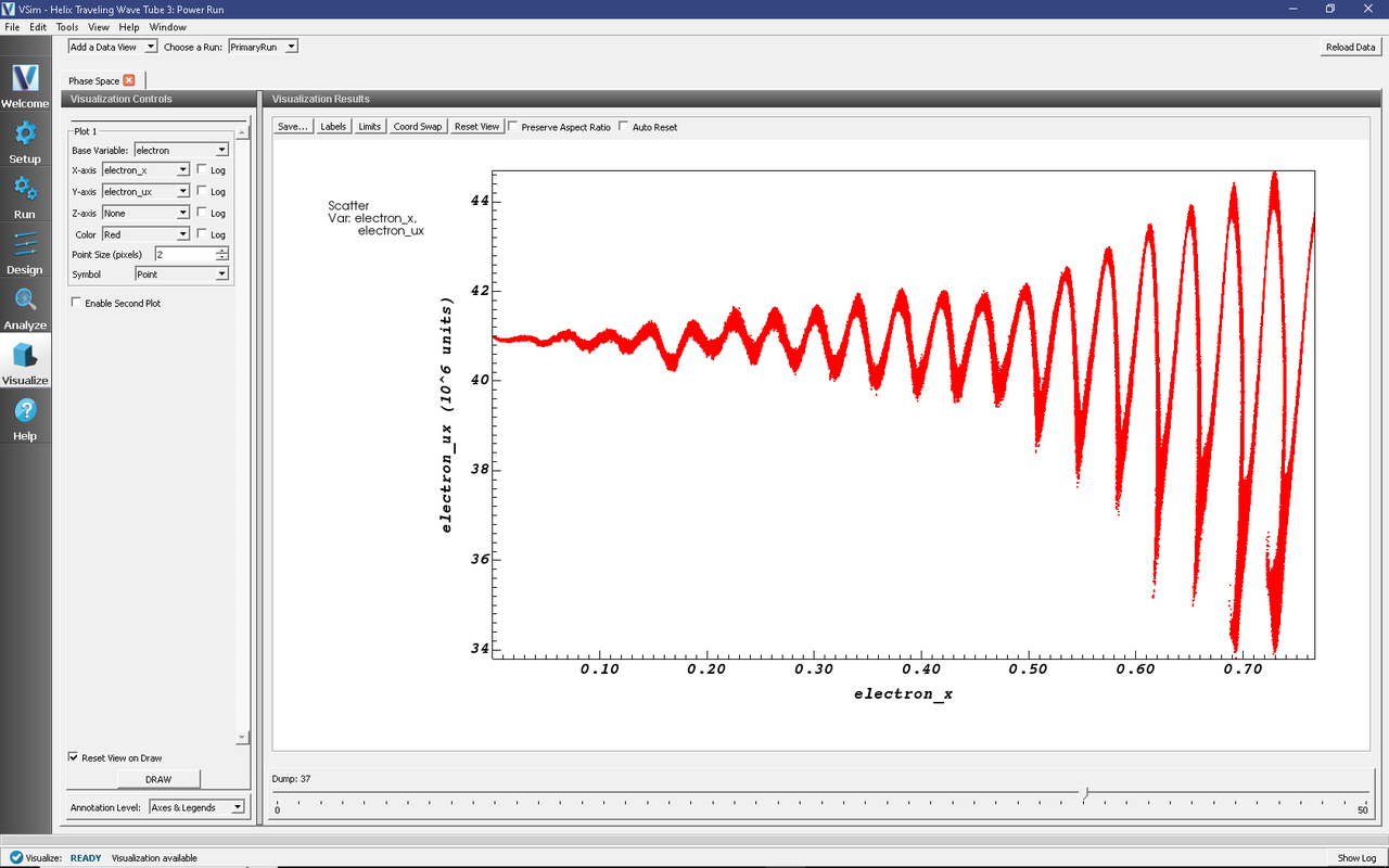
Fig. 435 Longitudinal phase space of the electron beam.

One can see in Fig. 435 that the beam has been overdriven, such that trapping is beginning to occur. Hence, one must either reduce the input power or one must reduce the gain. In the middle of the tube one can see that the beam oscillation for one cycle decays a bit before taking off again. This is where the attenuator is located.

The effect of overdriving the tube can also be seen in the longitudinal field, Fig. 436. This image is obtained by

For Data View select Field Analysis.
Set Field to E_x.
For Lineout Settings, choose Horizontal with Intercept of 0.
For Layout select Stacked 2d/1d.
Press Perform Lineout.
Click the Colors button and set the limits to Minimum = -2e3 and Maximum = 2e3.
Move the dump slider forward in time to see the evolution.
The image is at dump 37.

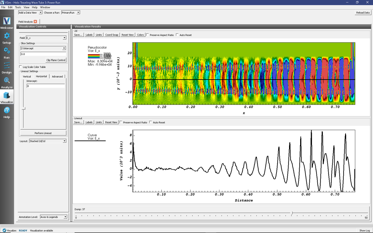
Fig. 436 Longitudinal electric field in the center of the tube.

As expected, the longitudinal field is largely confined within the helix. Again, at around x=0.4, one sees the field being damped out by the attenuator. Because the tube has been overdriven, harmonics are appearing in the field at the right. This image shows that the harmonics occur at about 1/5 of the current output power, indicating the amount by which one should decrease the input power or the gain to obtain linear operation.

The gain can be seen in the History records, which are available under the History Data View. A sample of these is shown in Fig. 437.

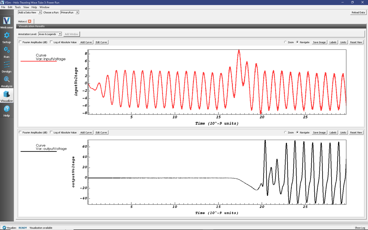
Fig. 437 Input and output voltage histories.

To obtain this history image:

For Data View select History.
For Graph 1 select inputVoltage.
For Graph 2 select outputVoltage.
For Graph 3 and Graph 4 select <None>

This image shows that the voltage gains is about a factor of 10 or 20 dB. The voltage history also shows the harmonics in the output that come from overdriving the tube.

Further Experiments

As noted at the beginning, this run could be run for many more time steps to determine whether backward oscillations are present. Additionally, one can experiment with the beam energy to determine what energy gives the most gain. Varying the input power can determine the maximum output power, which happens when the beam begins trapping at the end of the tube, or the input power at which one obtains large gain while remaining in the linear regime.