Antenna on Predator Drone (predatorDrone.sdf)
Keywords:
- predatorDrone, far field, radiation
Problem Description
This problem illustrates how to obtain the far field radiation patterns of a current source antenna mounted on a Predator Drone.
This simulation can be performed with a VSimEM license.
Opening the Simulation
The Predator Drone example is accessed from within VSimComposer by the following actions:
Select the New → From Example… menu item in the File menu.
In the resulting Examples window expand the VSim for Electromagnetics option.
Expand the Antennas option.
Select “Antenna on Predator Drone” and press the Choose button.
In the resulting dialog, create a New Folder if desired, and press the Save button to create a copy of this example.
The Setup Window is now shown with the CAD imported geometry and antenna current distribution accessible to the user. See Fig. 236.
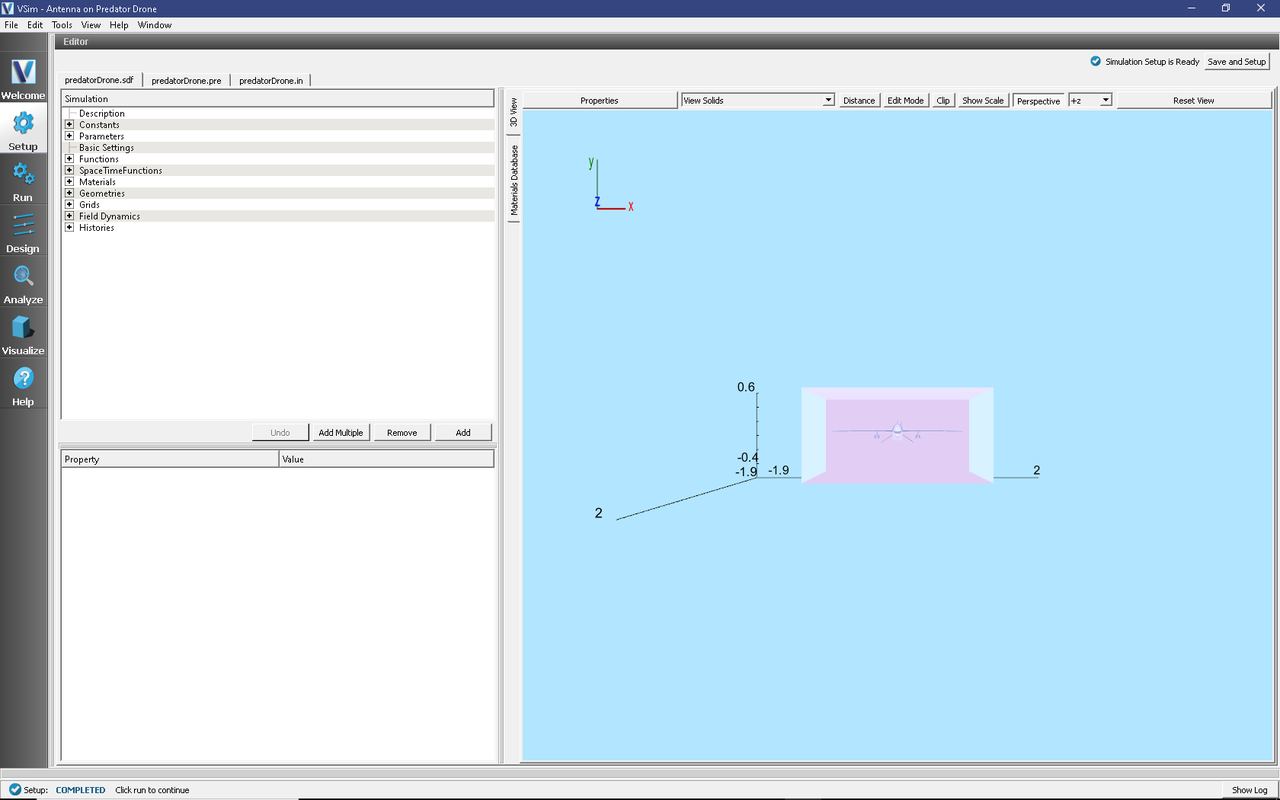
Fig. 236 Setup Window for the Predator Drone example.
One can click and unclick the grid, the farFieldBox0 in the histories, the current distribution, and so forth to see where those objects are. One can change locations through changing the values under Constants or, in some cases, the numbers directly in the objects.
Simulation Properties
This file allows the modification of antenna operating frequency, source amplitude, dimensions of the source and the Kirchhoff box by changing the associated variable values under the Constants.
Running the Simulation
After performing the above actions, continue as follows:
Proceed to the Run Window by pressing the Run button in the left column of buttons.
To run the file, click on the Run button in the upper left corner of the Logs and Output Files pane. You will see the output of the run in the right pane.
The run has completed when you see the output, “Engine completed successfully.” This is shown in Fig. 237.
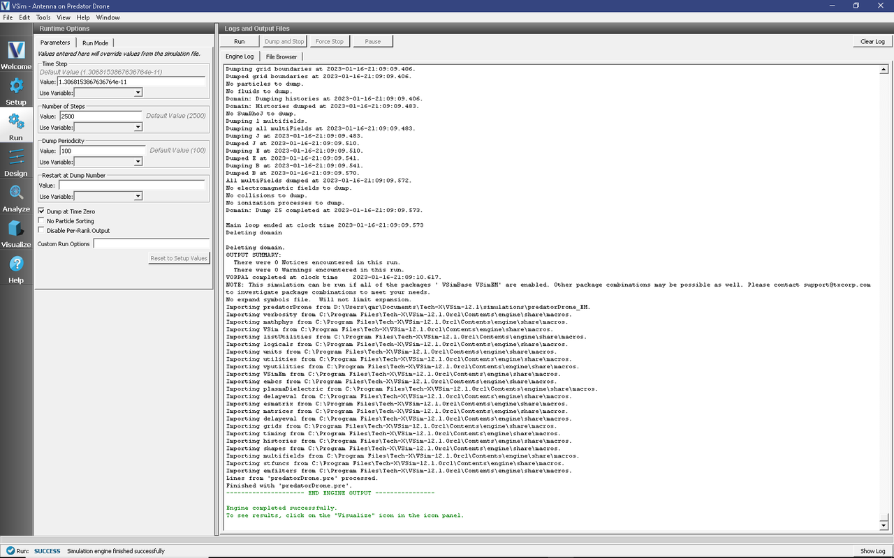
Fig. 237 The Run Window at the end of execution.
Analyzing the Results
After the run, one must analyze the Kirchhoff box data to get the far fields. This is done as follows:
Proceed to the Analysis window by pressing the Analyze button in the left column of buttons.
Click on computeFarFieldFromKirchhoffBox.py, then click on the Open button.
If you want, you can grab the dividing bar between the list of Analyzers in the Analysis Controls window and the Analysis Results window, and slide it left to cover up the Analysis Controls window, making more room for the Analysis Results window.
After performing the above actions continue as follows to compute the far field radiation pattern:
In the resulting list, select computeFarFieldFromKirchhoffBox and press Open
The analyzer fields should be filled as below:
simulationName: predatorDrone
fieldLabel: E
farFieldRadius: 1024.0
numPeriods: 0.25
numFarFieldTimes: 2
frequency: 1.0e9
numTheta: 45
numPhi: 60
zeroThetaDirection: (0,0,1)
zeroPhiDirection: (1,0,0)
incidentWaveAmplitude - blank
incidentWaveDirection - (0,0,0)
varyingMeshMaxRadius - 1024.0
principalPlanesOnly - checked
Click Analyze in the top right corner.
The analysis is completed when you see the output shown in Fig. 233.
If you want the script to run faster, lower numTheta to 8 and numPhi to 16.
Press the Analyze button in the top left of the window.
At completion, you will see Fig. 238. The far field data is written to vsh5 files in the simulation directory.
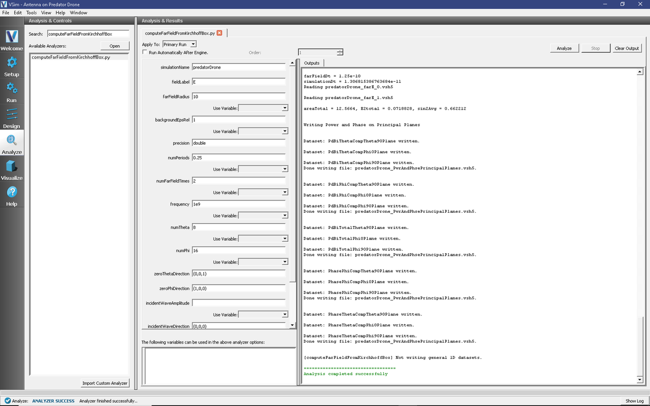
Fig. 238 The Analysis window at the end of execution.
Visualizing the Results
Proceed to the Visualize Window by pressing the Visualize button in the left column of buttons.
The radiation pattern in real space can be visualized by doing the following:
Expand Scalar Data
Expand E
Select one of the scalar fields, such as E_x
Check Clip Plot
Check Display Contours and set the number of contours to 10
Set minimum to -75 and maximum to 60
Click on Plane Controls, change only Plane3 and set Z to -1.
Expand Geometries
Check poly_surface (predatorGeomSolid)
Move the Dump slider to dump 15 to see the same far field as Fig. 239.
It is useful to reset the color minimum and maximum and change the number of Contours, to give a pleasing pattern, as shown in Fig. 239. An odd number of contours will result in a contour at zero field, which often leads to a less attractive plot with the zero contour filling up the space. Thus, in this case, an even number of contours is suggested.
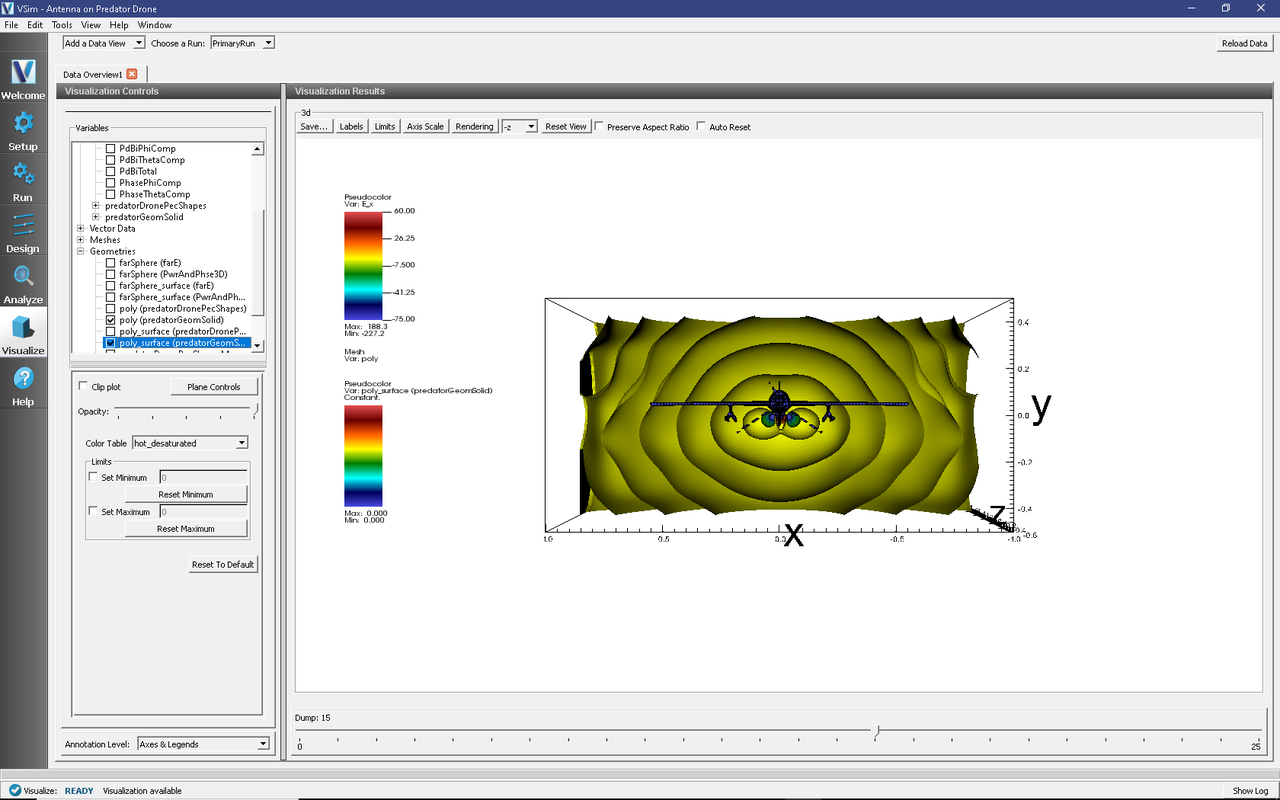
Fig. 239 The radiation pattern in real space
The far field radiation pattern, which was computed in the section on Analyzing the Results can also be displayed. Remove the previous image. Then check the PdBi box under Scalar Data, and move the dump slider to the beginning dump. You will see a 3D radiation surface, representing the Far Field radiation power level at each angle that was processed. Colors and radius are in units of dBi, decibels relative to isotropic. A notable peak in the radiation pattern is evident in the forward, upward, and downward directions, as seen in Fig. 240.
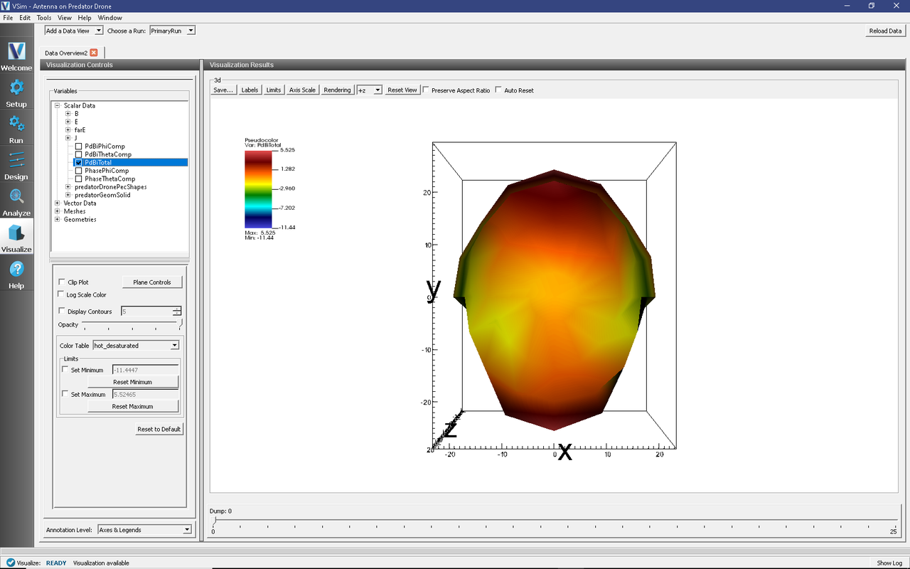
Fig. 240 The far field radiation pattern
Further Experiments
Upon close inspection you will note that the mesh size is slightly too large to fully resolve the thin wing structures of the tail section. You can experiment with smaller cell size to resolve these structures. Beware that more cells will increase the run time.
This example can be extended to meet any antenna placement problem with by addition of parameters to define the current distribution center. The vertical extent of the simulation box could be shrunk to reduce the simulation time, which would then allow greater resolution of the wavelength.
The main driver of simulation accuracy is the number of points per wavelength. Because of this lower frequencies will simulate in less time as they require fewer cells to achieve the same resolution in the wave.