2.4 GHz Yagi Uda Antenna (YagiUda2p4.sdf)
Keywords:
- yagiUdaArrayWireModel, yagiT, far field, radiation
Problem description
A Yagi-Uda array is a directional antenna consisting of several parallel dipole elements. Only one of these dipole elements is driven, the other elements being parasitic . Directionality is achieved by requiring that there be one longer element adjacent to the source element, which is referred to as the reflector. The rest of the elements being adjacent to the source but opposite to the reflector, and shorter than the source element, are referred to as directors. Yagi antennas are ubiquitous, and as such optimal parameters for dipole lengths and separations have been established. We go with values one would typically find in any text covering the matter. This example illustrates how to obtain the far field radiation pattern of a Yagi-Uda array.
This simulation can be performed with a VSimEM license.
Opening the Simulation
The Yagi-Uda example is accessed from within VSimComposer by the following actions:
Select the New → From Example… menu item in the File menu.
In the resulting Examples window expand the VSim for Electromagnetics option.
Expand the Antennas option.
Select 2.4 GHz Yagi Uda Antenna and press the Choose button.
In the resulting dialog, create a New Folder if desired, and press the Save button to create a copy of this example.
All of the properties and values that create the simulation are now available in the Setup Window as shown in Fig. 184. You can expand the tree elements and navigate through the various properties, making any changes you desire. The right pane shows a 3D view of the geometry, if any, as well as the grid, if actively shown. To show or hide the grid, expand the Grids element and select or deselect the box next to Grid.
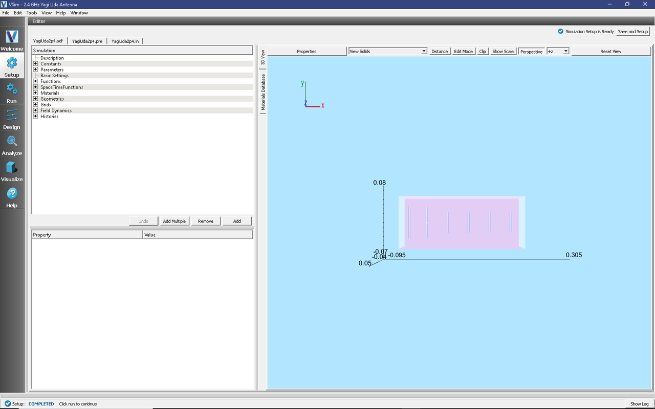
Fig. 184 Setup Window for the Yagi-Uda example.
Simulation Properties
This file allows the modification of the antenna operating frequency, antenna dimensions, and simulation domain size.
By adjusting the dimensions any sized Yagi-Uda array can be simulated.
Note
To obtain good far field resolution generally four or more antenna elements is desirable (One source, one reflector, two or more directors).
Running the Simulation
After performing the above actions, continue as follows:
Proceed to the Run Window by pressing the Run button in the left column of buttons.
Here you can set run parameters, including how many cores to run with.
When you are finished setting run parameters, click on the Run button in the upper left corner of the Logs and Output Files pane. You will see the output of the run in the right pane. The run has completed when you see the output, “Engine completed successfully.” This is shown in Fig. 185.
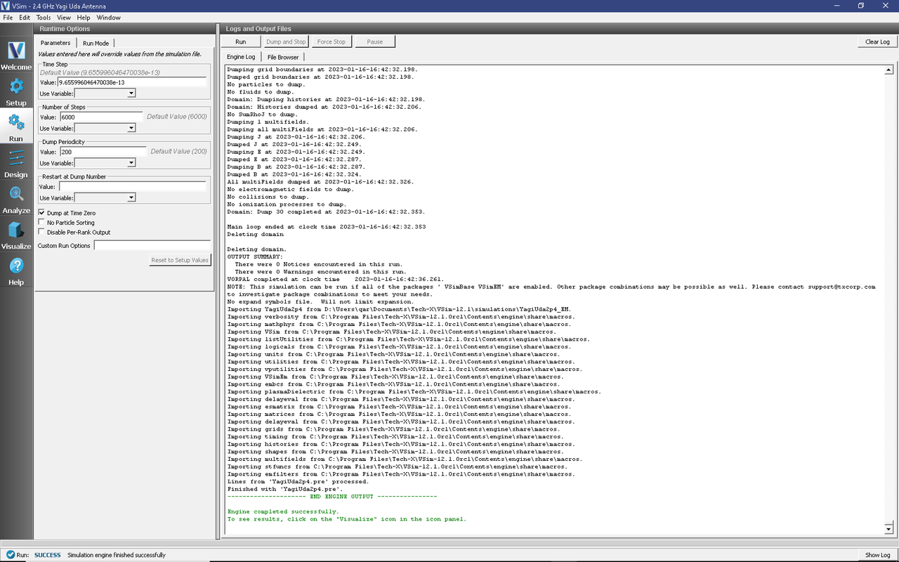
Fig. 185 The Run Window at the end of execution.
Analyzing the Results
Proceed to the Analysis window by pressing the Analyze button in the left column of buttons.
Select computeFarFieldFromKirchhoffBox.py from the list and select “Open” (Fig. 186)
Input values for the analyzer parameters. The analyzer may be run multiple times, allowing the user to experiment with different values.
simulationName - yagiUda2p4
fieldLabel - E
farFieldRadius - 1024.0
numPeriods - 0.25
numFarFieldTimes - 2
frequency - 2.4e9
numTheta - 45
numPhi - 60
zeroThetaDirection - (0,1,0)
zeroPhiDirection - (0,0,1)
incidentWaveAmplitude - blank
incidentWaveDirection - (0,0,0)
varyingMeshMaxRadius - 1024.0
principalPlanesOnly - checked
Click “Analyze”
Depending on the values of numTheta, numPhi, and numFarFieldTimes, the script may need to run for several minutes.
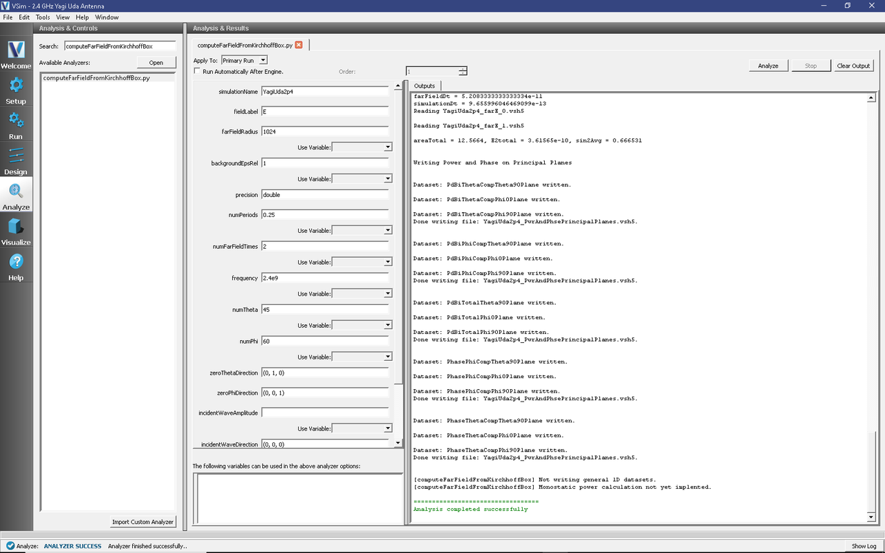
Fig. 186 The Analysis Window.
Visualizing the results
Proceed to the Visualize Window by pressing the Visualize button in the left column of buttons.
To view the near field pattern, do the following:
Expand Scalar Data
Expand E
Select E_x
Check the Set Minimum box and set the value to -0.1
Check the Set Maximum box and set the value to 0.1
Check the Clip Plot box
Expand Geometries
Select poly (YagiUda2p4PecShapes)
Move the dump slider forward in time
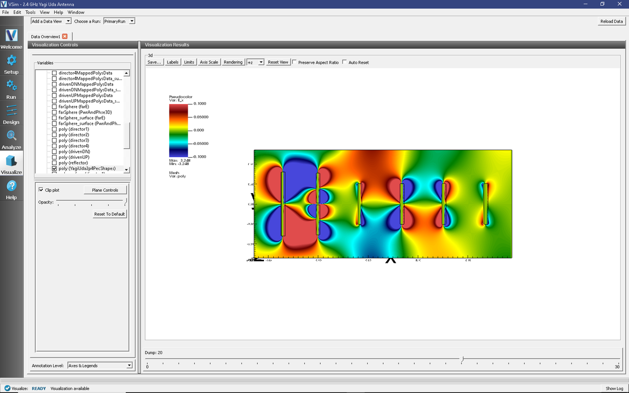
Fig. 187 The electric field near-field pattern.
The far field radiation pattern can be found in the scalar data variables of the data overview tab underneath the farE field. Uncheck the E_x dataset and check the farE_magnitude box under farE.
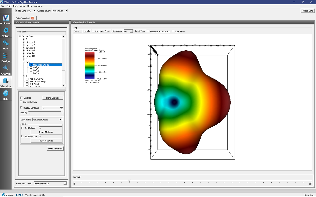
Fig. 188 The electric field manifestation of the far field pattern.
Further Experiments
Try adding more directors and changing their dimensions to see the effect on the far field pattern.