Horn Antenna (hornAntenna.sdf)

Keywords:

sectoral, horn antenna, far field, radiation

Problem description

This example illustrates how to obtain the far field radiation pattern of a sectoral horn antenna. A horn antenna consists of a flaring metal waveguide shaped like a horn that directs radio waves into a beam. Horns are widely used as antennas at UHF and microwave frequencies. A sectoral horn is only flared along one axis, the other horn axis has constant width and is equivalent to the width of the waveguide. Sectoral horns produce a fan shaped beam, wider in the plane of the narrow sides.

This simulation can be run with a VSimEM license.

Opening the Simulation

The Horn Antenna example is accessed from within VSimComposer by the following actions:

• Select the New → From Example… menu item in the File menu.

• In the resulting Examples window expand the VSim for Electromagnetics option.

• Expand the Antennas option.

• Select “Horn Antenna” and press the Choose button.

• In the resulting dialog, create a New Folder if desired, and press the Save button to create a copy of this example.

The Setup Window is shown Fig. 222. One can click and unclick the grid, the farFieldBox0 in the histories, the current distribution, and so forth to see where those objects are. One can change locations through changing the values under Constants or, in some cases, the numbers directly in the objects.

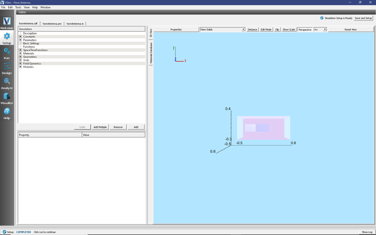
Fig. 222 Setup Window for the Horn Antenna example.

Simulation Properties

The antenna geometry in this example has been set up using CSG in the graphical setup interface. The dimensions of the antenna can be adjusted by tuning the sizes of the various wedges and cubes used in the antenna’s construction. Under Constants, the wavelength may be modified, as well as the grid size and resolution. The polarization of the antenna may be altered by going into CurrentDistributions and changing the components of the driving current source.

There are two scales that we need to resolve in this simulation. One is the wavelength and one is the smallest geometric scale to resolve (i.e. in this simulation it is the wall width). So, NX, NY, and NZ have been set up to resolve both scales.

Running the Simulation

Once finished with the problem setup, continue as follows:

• Proceed to the Run Window by pressing the Run button in the left column of buttons.

• Choose parallel computing options on the MPI tab.

• To run the file, click on the Run button in the upper left corner of the Logs and Output Files pane. You will see the output of the run in that pane. The run has completed when you see the output, “Engine completed successfully.” This is shown in the window below.

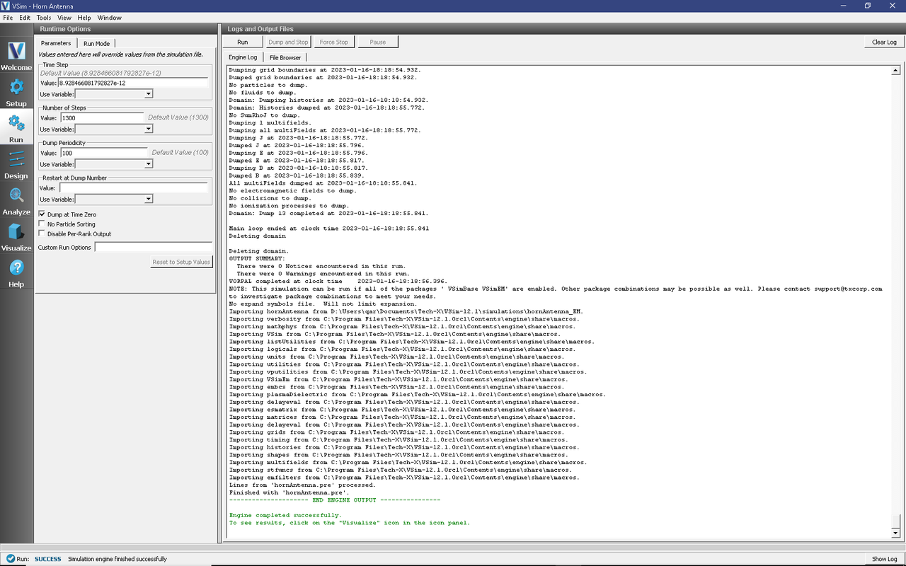
Fig. 223 The Run Window at the end of execution.

Analyzing the Results

After performing the above actions, continue as follows:

• Proceed to the Analysis window by pressing the Analyze button in the left column of buttons.

• In the resulting dialog, select computeFarFieldFromKirchhoffBox.py and press Open.

• Input values for the analyzer parameters. The analyzer may be run multiple times, allowing the user to experiment with different values.

  • simulationName - hornAntenna (name of the input file)

  • fieldLabel - E (name of the electric field)

  • farFieldRadius - 10.0 (distance to far field in m, 10.0 is a good value)

  • numPeriods - 0.25

  • numFarFieldTimes - 2

  • frequency - 2.0e9

  • numTheta - 45 (number of theta points in the far field, 18 for a quick calculation, 45 for finer resolution)

  • numPhi - 90 (number of phi points in the far field, 36 for a quick calculation, 90 for finer resolution)

  • zeroThetaDirection - (0,0,1) (determines orientation of far field coordinate system)

  • zeroPhiDirection - (1,0,0) (determines orientation of far field coordinate system

  • incidentWaveAmplitude - blank

  • incidentWaveDirection - (0,0,0)

  • varyingMeshMaxRadius - 10.0

  • principalPlanesOnly - checked

• Click Analyze

• The analysis is completed when you see “Analysis completed successfully” in the Outputs. Depending on the values of numTheta, numPhi, and timeStepStride, the script may need to run for several minutes or longer.

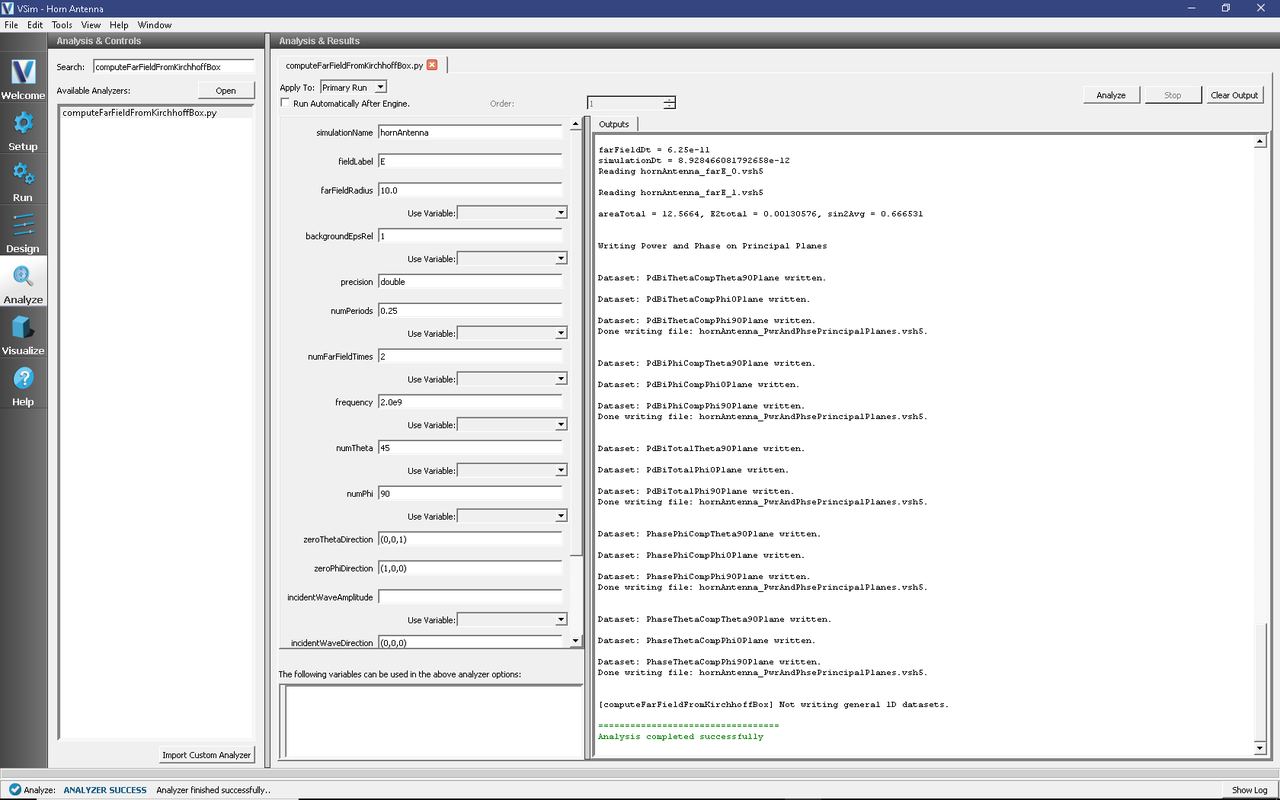
Fig. 224 The Analyze panel after running computeFarFieldFromKirhhoffBox.py.

Visualizing the Results

Under Scalar Data plot \(E_{magnitude}\). To slice inside the horn, select Clip Plot in the lower left hand corner. Click on Plane Controls and change the cut-plane normal to lie along Y instead of Z. Move the dump slider to view the electric field emanating from the horn. You can get a better look by adjusting the color scale. Select Log Scale Color in the lower left hand corner. Try adjusting the min and max until the signal is well resolved (see Fig. 225).

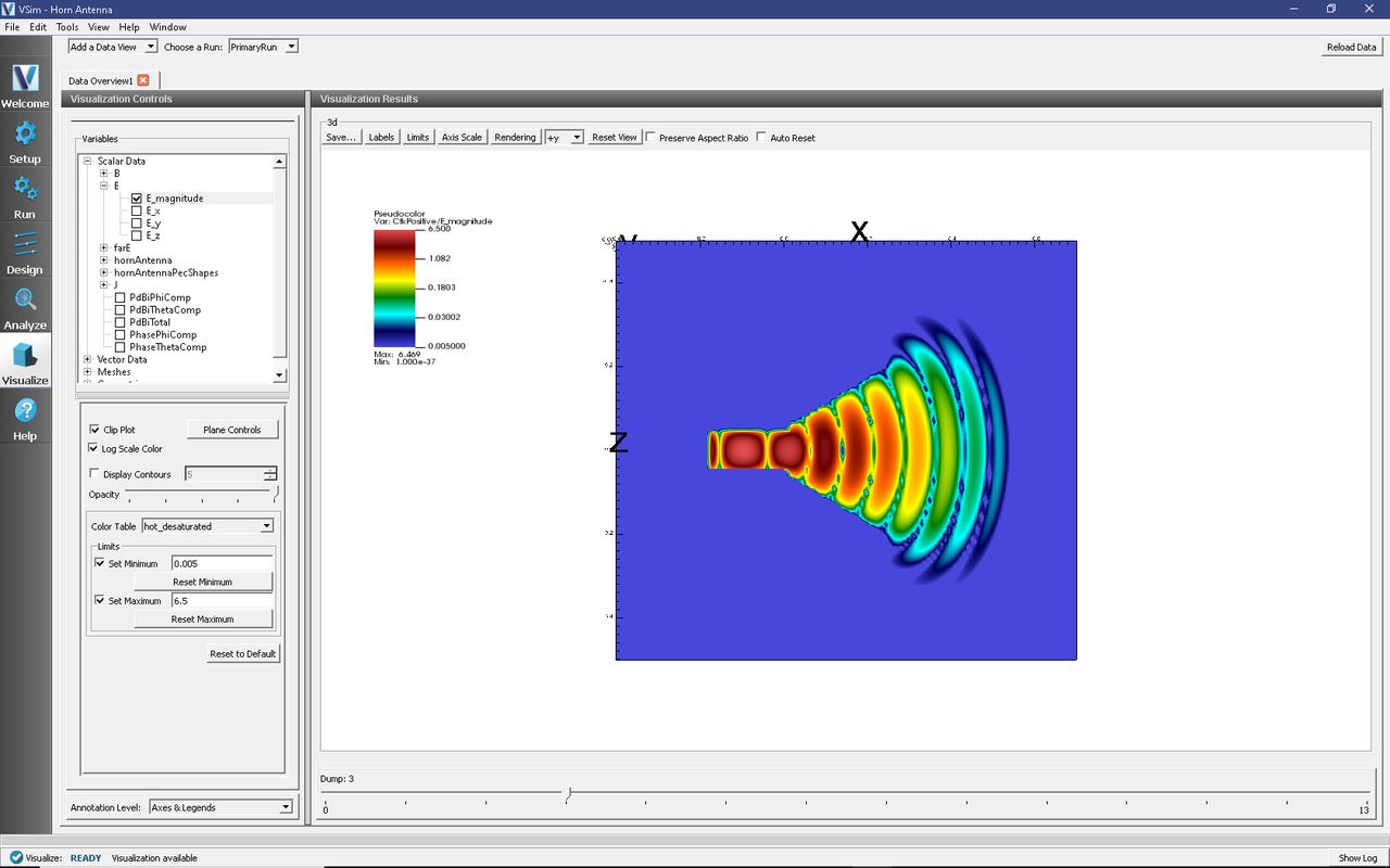
Fig. 225 The \(E_{magnitude}\) field propagating out of the horn at dump 3. The color scale has been log scaled and the min and max have been fixed to 0.005 and 6.5, respectively. The optimal min/max values will depend on the dump selected. The view has been rotated to show the x-z plane.

The far field radiation pattern can be found in the Scalar Data variables of the Data Overview tab. Open the farE tree element and check the farE_magnitude box. The far field mesh can also be plotted; it can be found under Geometries.

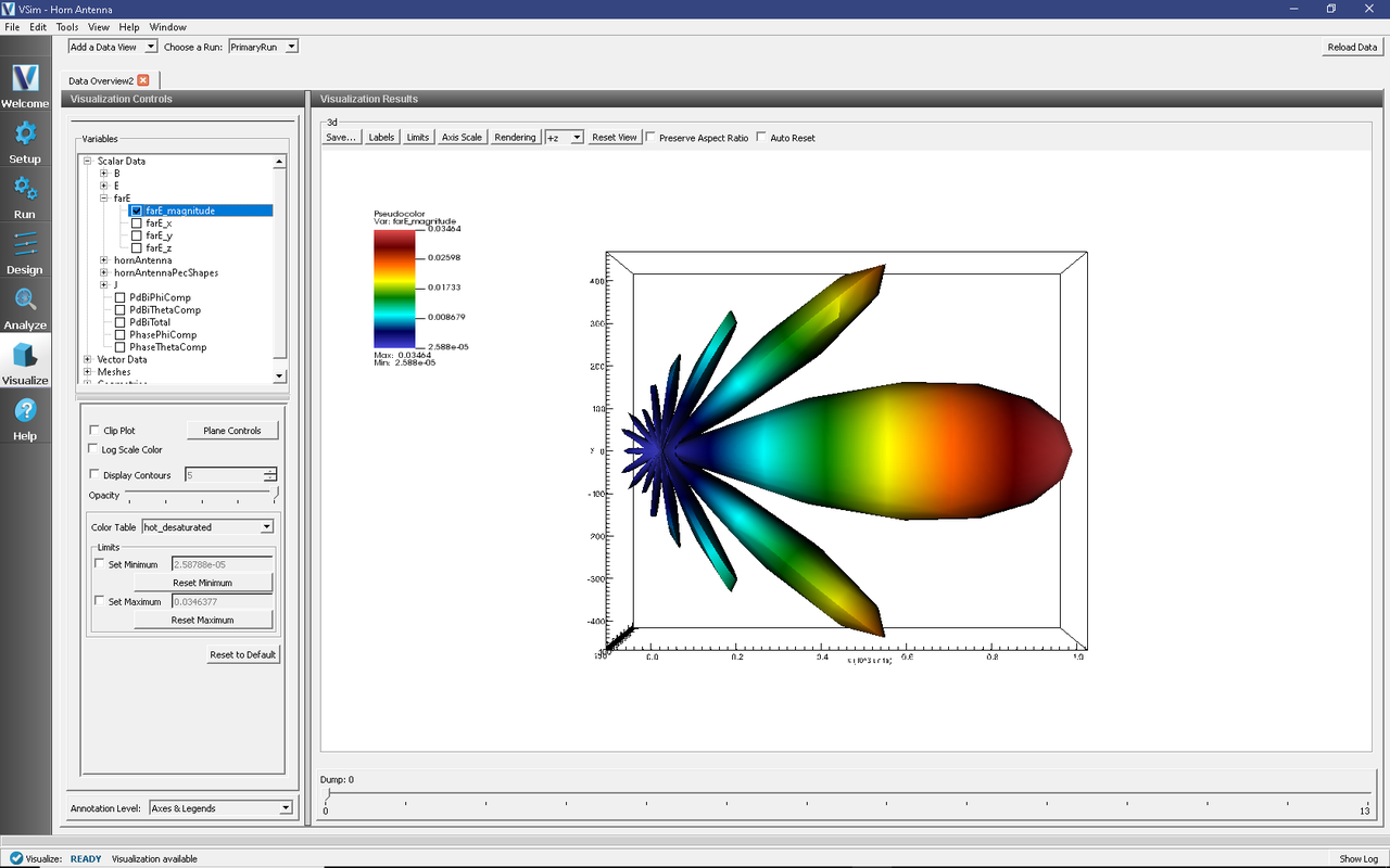
Fig. 226 The far field radiation pattern.

Further Experiments

The physical dimensions of the pyramidal horn can be modified in the GUI.

To turn the antenna into an E-plane sectoral horn, try changing the polarization to lie along the flared direction (z).

Try experimenting with different far field resolutions by changing the values of numTheta and numPhi during the Analyze step. You can also experiment with different far field distances by changing the value of farFieldRadius.

Try making the domain and the size of the Kirchhoff box larger or smaller (size of the Kirchhoff box is tied to the domain size by default). If the simulation domain is made too small, the results may appear distorted because the entire near field must be resolved within the simulation domain in order to achieve a proper transformation to the far field.