Like-Charge Dipole (esChargedSpheres.sdf)

Keywords:

electrostatics, like-charge dipole

Problem description

This Like-Charge Dipole simulation computes the electrostatic potential and field for a dipole of two spheres with given radius at the same potential.

This simulation can be performed with a VSimEM or VSimPD license, with Composer licensed for Visual Setup.

Opening the Simulation

The Like-Charge Dipole example is accessed from within VSimComposer by the following actions:

• Select the New → From Example… menu item in the File menu.

• In the resulting Examples window expand the VSim for Electromagnetics option.

• Expand the Electrostatics option.

• Select Like-Charge Dipole and press the Choose button.

• In the resulting dialog, create a New Folder if desired, and press the Save button to create a copy of this example.

All of the properties and values that create the simulation are now available in the Setup Window as shown in Fig. 241. You can expand the tree elements and navigate through the various properties, making any changes you desire. The right pane shows a 3D view of the geometry, if any, as well as the grid, if actively shown. To show or hide the grid, expand the Grid element and select or deselect the box next to Grid.

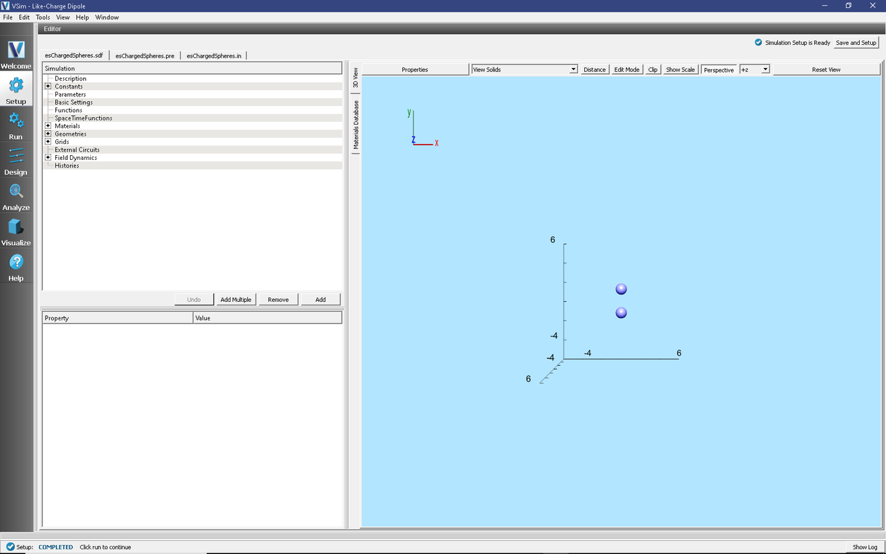
Fig. 241 Setup Window for the Like-Charge Dipole example.

Simulation Properties

This simulation uses visual setup to create a simple dipole. To do this we employ a few simple techniques such as Constructive Solid Geometries (CSG), and field Boundary Conditions. The dipole is constructed as two spheres of identical size. A Dirichlet boundary condition with the desired voltage is applied on both spheres.

Running the simulation

After performing the above actions, continue as follows:

• Proceed to the Run Window by pressing the Run button in the left column of buttons.

• To run the file, click on the Run button in the upper left corner of the Logs and Output Files pane. You will see the output of the run in this pane. The run has completed when you see the output, “Engine completed successfully.” This is shown in Fig. 242.

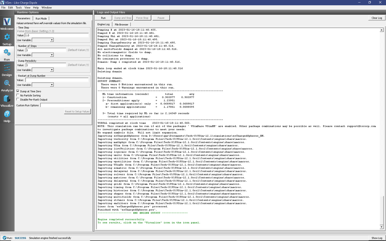
Fig. 242 The Run Window at the end of execution.

Visualizing the results

After performing the above actions, continue as follows:

• Proceed to the Visualize Window by pressing the Visualize button in the left column of buttons.

To view the electrostatic potential of the dipole as seen in Fig. 243 do the following:

• Expand Scalar Data

• Select Phi

• Select Display Contours

• Select Clip Plot

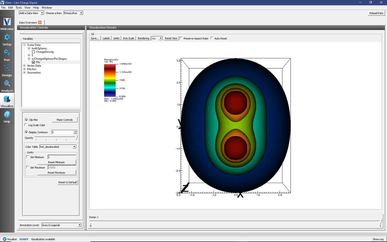
Fig. 243 Visualization of Like-Charge Dipole as a pseudocolor plot.

Further Experiments

Change the distance between spheres and see how the electric field changes.

Change the sphere radius and see how the electric field changes.

Change the sphere’s potential to observe a change in the electric field.

Determine how the electric field changes with varying resolution.