Dipole Above Conducting Plane (dipoleOnConductingPlane.sdf)
Keywords:
- dipoleOnConductingPlane, far field, radiation
Problem Description
This problem illustrates how to obtain far fields within VSim by simulating an infinitesimally short dipole mounted a variable height above a conducting plane. The conducting plane is simulated by using the method of images and utilizes an equal magnitude dipole with direction rotated azimuthally by PI, on the opposite side of the plane. This example is similar to the Oscillating Dipole Above Conducting Plane of VSimBase, but modified with functionality available as part of the VSimEM package to obtain the far field radiation pattern. The number of lobes in the far field will vary as a function of height above the conducting plane. There will be 2*HEIGHT/WAVELENGTH + 1 lobes.
This simulation can be performed with a VSimEM license.
Opening the Simulation
The Dipole Above Conducting Plane example is accessed from within VSimComposer by the following actions:
Select the New → From Example… menu item in the File menu.
In the resulting Examples window expand the VSim for Electromagnetics option.
Expand the Antennas option.
Select “Dipole Above Conducting Plane” and press the Choose button.
In the resulting dialog, create a New Folder if desired, and press the Save button to create a copy of this example.
All of the properties and values that create the simulation are
now available in the Setup Window as shown in
Fig. 211. You can expand the
tree elements and navigate through the various properties, making
any changes you desire. The right pane shows a 3D view of the
geometry, if any, as well as the grid, if actively shown. To show
or hide the grid, expand the Grid element and select or deselect
the box next to Grid.
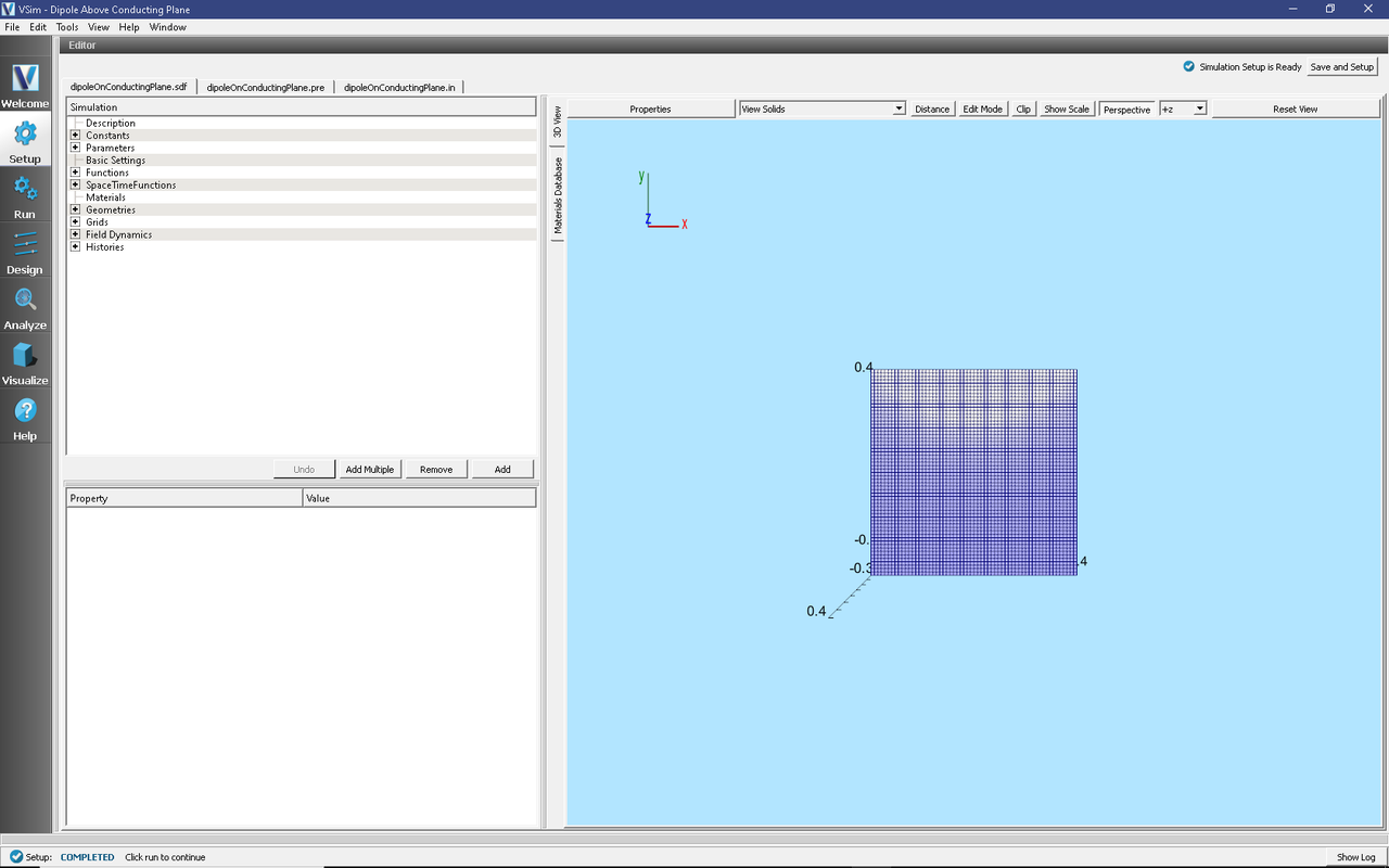
Fig. 211 Setup Window for the Dipole Above Conducting Plane example.
Simulation Properties
This setup includes several Constants and Parameters to help define the dipole signals, including the frequency and height of the antenna.
There are open boundary conditions on each side of the simulation domain.
The conducting plane is simulated by using the method of images and utilizes an equal magnitude dipole with direction rotated azimuthally by PI, on the opposite side of the plane.
Running the Simulation
After performing the above actions, continue as follows:
Proceed to the Run Window by pressing the Run button in the left column of buttons.
To run the file, click on the Run button in the upper left corner of the window. You will see the output of the run in the right pane. The run has completed when you see the output, “Engine completed successfully.” This is shown in Fig. 212.
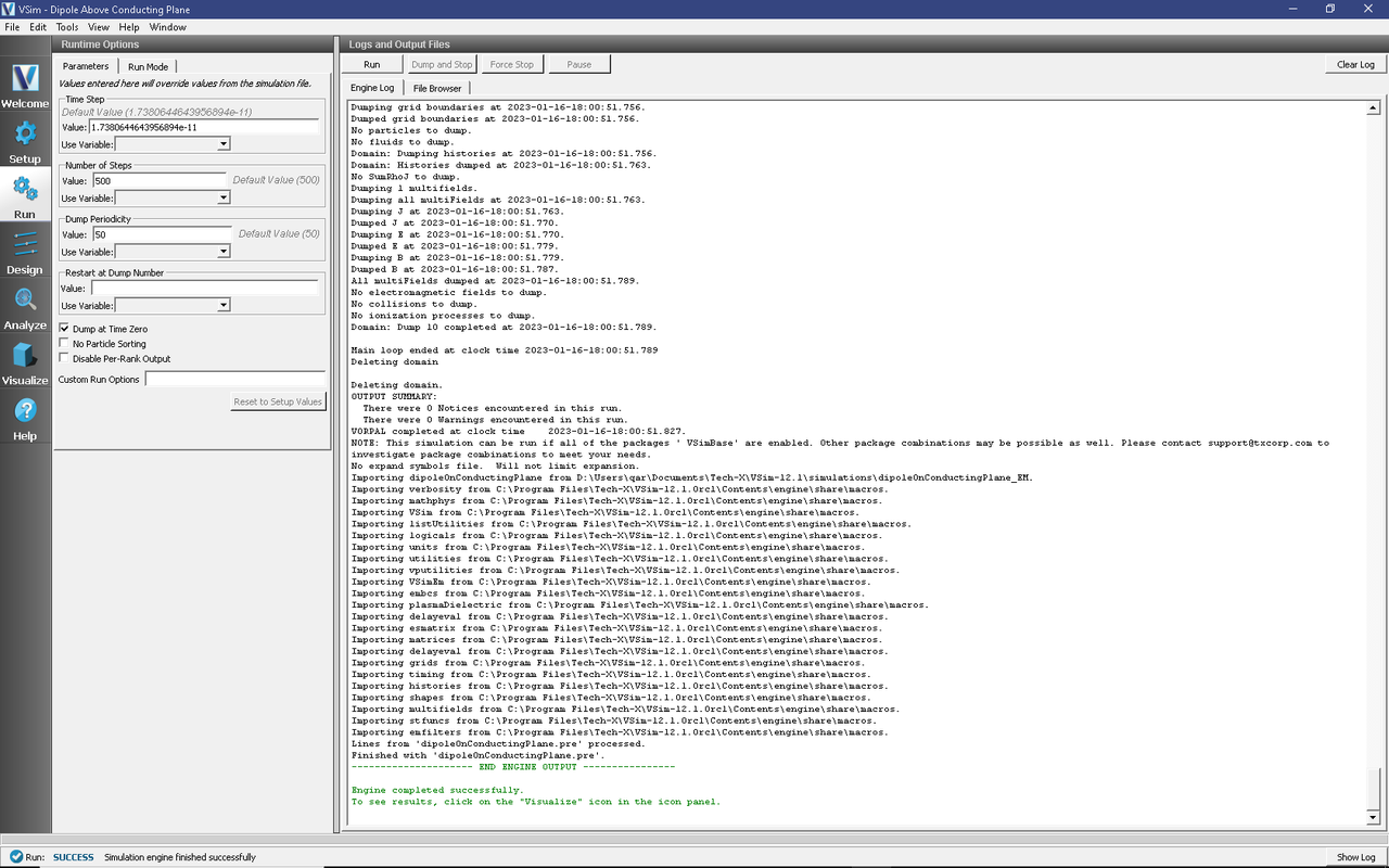
Fig. 212 The Run Window at the end of execution.
Analyzing the Results
Proceed to the Analysis window by pressing the Analyze button in the left column of buttons.
Select the Default computeFarFieldFromKirchhoffBox.py Analyzer
Input values for the variables given on the left hand side of the screen. Check that these have the following values:
simulationName - dipoleOnConductingPlane (name of the input file)
fieldLabel - E
farFieldRadius - 1024.0
numPeriods - 0.25
numFarFieldTimes - 2
frequency - 3.0e9
numTheta - 45 (number of points in the theta direction)
numPhi - 90 (number of points in the phi direction)
zeroThetaDirection - (0,0,1)
zeroPhiDirection - (1,0,0)
incidentWaveAmplitude - blank
incidentWaveDirection - (0,0,0)
varyingMeshMaxRadius - 1024.0
principalPlanesOnly - checked
Click the Analyze button near the top right of the window.
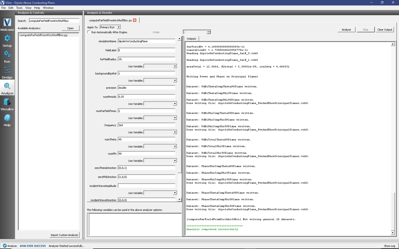
Fig. 213 The Analyze Window at the end of execution.
Visualizing the Results
The far field radiation pattern can be found in the Scalar Data variables of the data overview tab. Expand farE and then check the farE_magnitude box. You may need to rotate the view and check the Clip Plot box to hide the virtual far field pattern under the conducting plane.
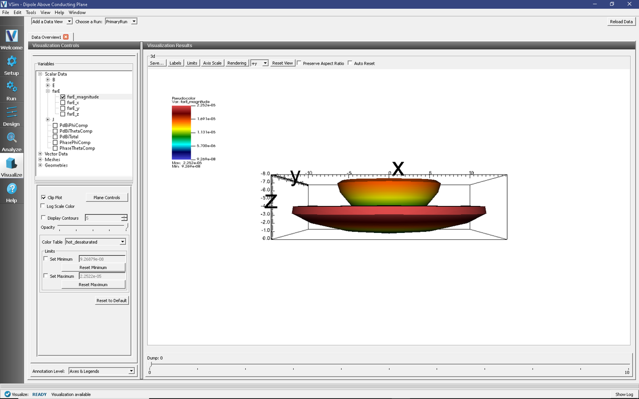
Fig. 214 The far field radiation pattern
Further Experiments
The number of lobes in the far field is dependent on Antenna Orientation and height. If vertically oriented there will be 2*Height/Wavelength +1 lobes. A horizontally oriented dipole will produce 2*Height/Wavelength lobes.
The resolution of the far field pattern can be changed by editing the number of theta and phi points in the analysis.
If the Simulation domain is made too small, the results will be distorted as the entire near field must be within the simulation domain in order to achieve a proper transformation to the far field.
Note that an infinite perfect electric conducting plane is simulated in the computational engine via image theory. An equal infinitesimal dipole is placed the same distance from the conducting “plane” in order to achieve the result of having an infinite electric conductor.