Loop Antenna from a Coaxial Cable (coaxialLoopAntenna.sdf)
Keywords:
- coaxial, coaxial waveguide, coaxial cable
Problem description
This example illustrates how to use the coaxial cable Field Boundary Condition and Constructive Solid Geometry to create a coaxial loop antenna.
This simulation can be run with a VSimEM, VSimVE, VSimPD, or VSimPA license.
Opening the Simulation
The Coaxial Loop Antenna example is accessed from within VSimComposer by the following actions:
Select the New → From Example… menu item in the File menu.
In the resulting Examples window expand the VSim for Electromagnetics option.
Expand the Antennas option.
Select “Loop Antenna From a Coaxial Cable” and press the Choose button.
In the resulting dialog, create a New Folder if desired, and press the Save button to create a copy of this example.
The Setup Window is shown Fig. 204.
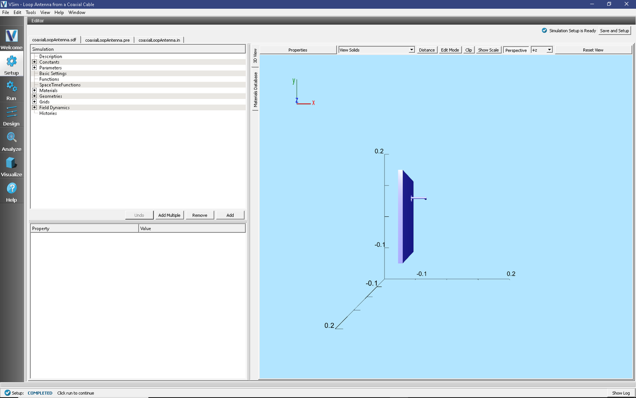
Fig. 204 Setup Window for the Coaxial Loop Antenna example.
Simulation Properties
This simulation makes use of the new coaxial waveguide Field Boundary Condition in VSim 8.1.
A coaxial waveguide is first constructed by creating a physical coaxial cable that enters the simulation domain. It is very important that this cable exists from at least 1 cell outside of the simulation boundary to 1 cell inside the simulation boundary. This is done by first creating a box primitive and setting it along the desired simulation boundary.
A cylinder corresponding to the outer diameter of the coaxial cable is then created, and subtracted from the plate.
A cylinder corresponding to the inner diameter of the coaxial cable is then created and extended into the simulation space.
It is then made into a loop antenna by adding a second, intersecting cylinder.
The wave itself is specified by a Field Boundary Condition.
Running the Simulation
Once finished with the problem setup, continue as follows:
Proceed to the Run Window by pressing the Run button in the left column of buttons.
Select appropriate settings in the Parameters and Run Mode sections
To run the file, click on the Run button in the upper left corner of the Logs and Output Files pane. You will see the output of the run in this pane. The run has completed when you see the output, “Engine completed successfully.”
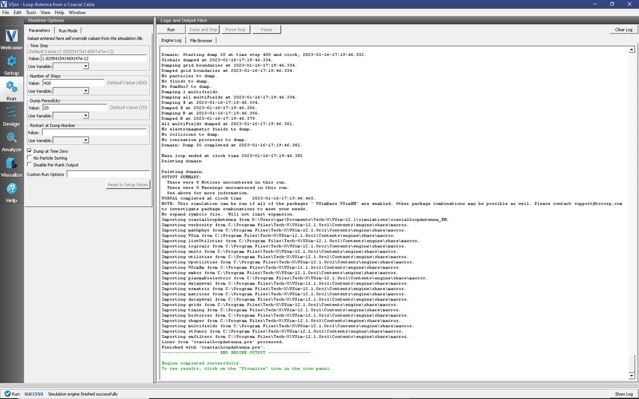
Fig. 205 The Run Window at the end of execution.
Visualizing the Results
After the run completes, the field may be visualized:
Proceed to the Visualize Window by pressing the Visualize button in the left column of buttons.
Expand Scalar Data, expand E, and select E_z.
To slice inside the field, select Clip Plot in the lower left hand corner, then click on Plane Controls and change the clip plane normal to Y instead of Z, and adjust the origin of the normal vector to Y = 0.05.
To adjust the colors, check the Set Minimum and Set Maximum boxes, and set the minimum to -10 and the maximum to 10.
Drag the Dump slider to the far right for dump 20.
Finally, click and drag the visualization to rotate it so that you can see the field.
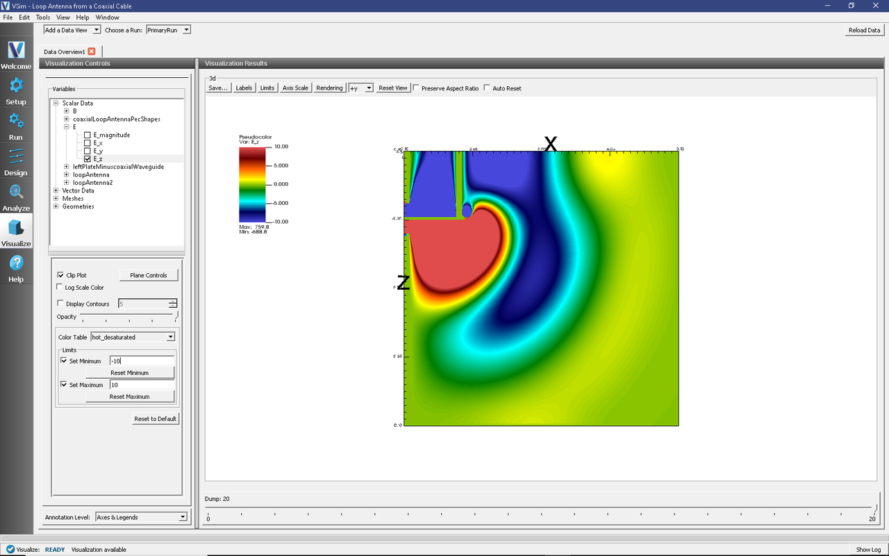
Fig. 206 The \(E_{z}\) field propagating off of the loop antenna.