Antenna Array 2D (antennaArray2D.sdf)
Keywords:
- antennaArray2D, far field, radiation, s-parameters
Problem Description
This set of 2-D VSimEM simulations shows how to obtain the far fields, S11 parameter, gain, and phase shift of a one-element antenna as well as the far fields, gain, S parameters, and phase shift of a multiple-element antenna array with one excited element. These simulations can be used as a basis for measuring coupling in phased array antennas. The analyzer compute2DantennaGainAndPhase.py is set up to calculate the S parameter for the excited element and any other reference element defined by the constant S_PARAM_ELEM.
This simulation can be run with a VSimEM license.
Opening the Simulation
The Antenna Array 2D example is accessed from within VSimComposer by the following actions:
Select the New → From Example… menu item in the File menu.
In the resulting Examples window expand the VSim for Electromagnetics option.
Expand the Antennas option.
Select Antenna Array 2D and press the Choose button.
In the resulting dialog, create a New Folder if desired, then press the Save button to create a copy of this example.
The resulting Setup Window is shown Fig. 189.
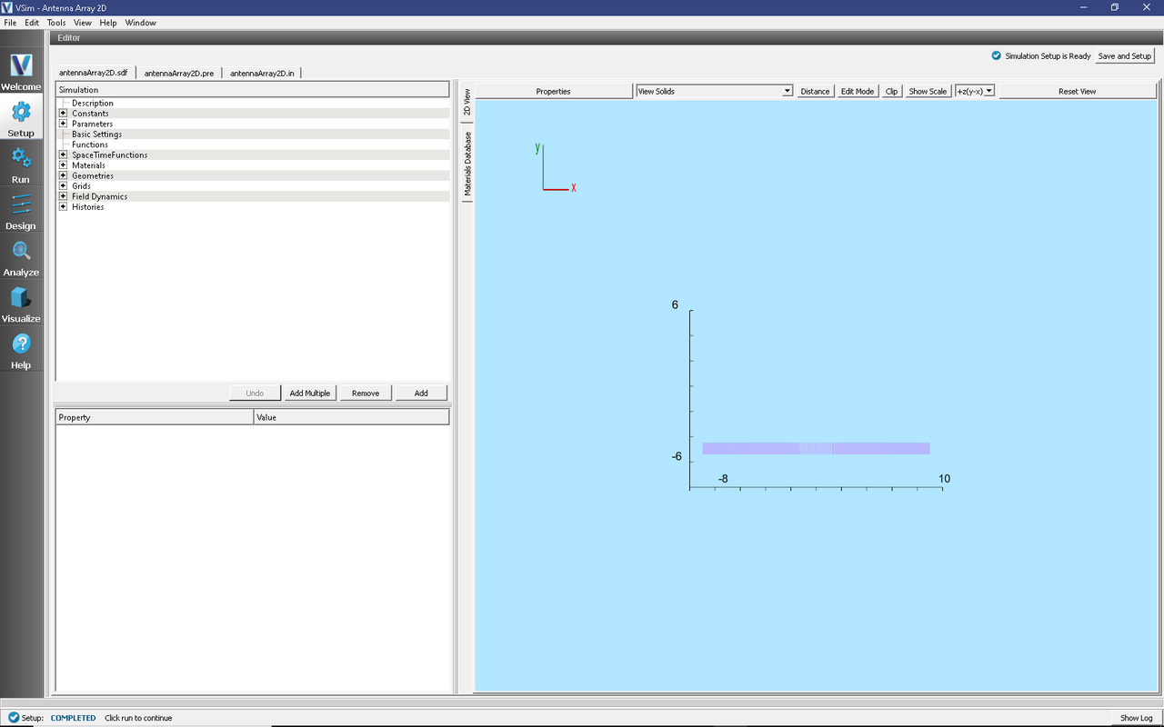
Fig. 189 Setup Window for the Antenna Array 2D example.
Simulation Properties
The antennas are waveguide apertures excited with a frequency of 1 GHz and the aperture width is \(0.1\lambda\) (see the parameter GAP in the element tree). The distance between the gaps is \(0.4\lambda\).
A different array of geometries can be created using input parameters such as number of elements in the array (N_ELEM) and the distance between the elements in each direction. To recreate a different antenna array, expand Geometries, expand CSG, right-click on gap → Create Array. In the Array Description window, select the “Union elements” checkbox, type in the number of elements to the value under N_ELEM, and the distance between elements to the value under DIST_ELEM. Then select the CSG “metal”, hold down Ctrl and select gapElemUnion located at the end of the gap array elements → Boolean Operation → select metal_gapElemUnion. Rename accordingly and assign the material PEC to the newly created geometry.
Running the Simulation
Once finished with the setup, continue as follows:
Proceed to the Run Window by pressing the Run button in the navigation column out left.
To run the file, click on the Run button in the upper left corner of the Logs and Output Files pane. You will see the output of the run in that pane. The run has completed successfully when you see the output, “Engine completed successfully.”
First run settings (default): * Number of Steps: 6000 * Dump Periodicity: 3000 * Dump at Time Zero: box checked
After the first run completes, proceed as follows:
Second run settings: * Change *Number of Steps to 1800 * Change *Dump Periodicity to 45 (Value taken from the parameter DUMP_PER_SECOND_RUN) * Set *Restart at Dump Number to 2
Note
If the grid properties change, these values will have to be adjusted.
The end of the second run is shown in Fig. 190.
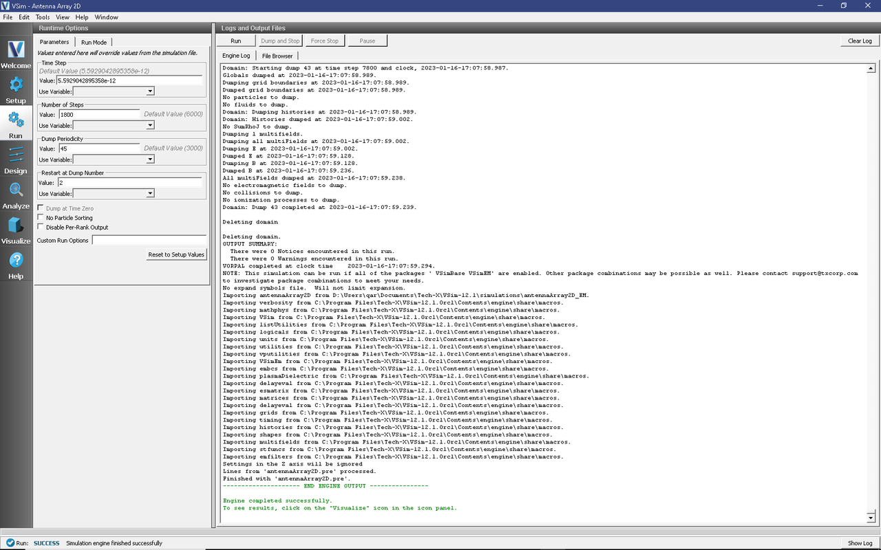
Fig. 190 The Run Window at the end of the second run execution.
Visualizing the Results
After performing the above actions, the results can be visualized as follows:
Proceed to the Visualize Window by pressing the Visualize button in the navigation column
Expand Scalar Data in the Visualization Controls pane
Expand E
Select E_x
Check the box for Set Minimum and set it to -100
Check the box for Set Maximum and set it to 100
Select the dump slider and move it to higher dump numbers to see the evolution of the electric field in time.
The resulting visualization is shown in Fig. 191.
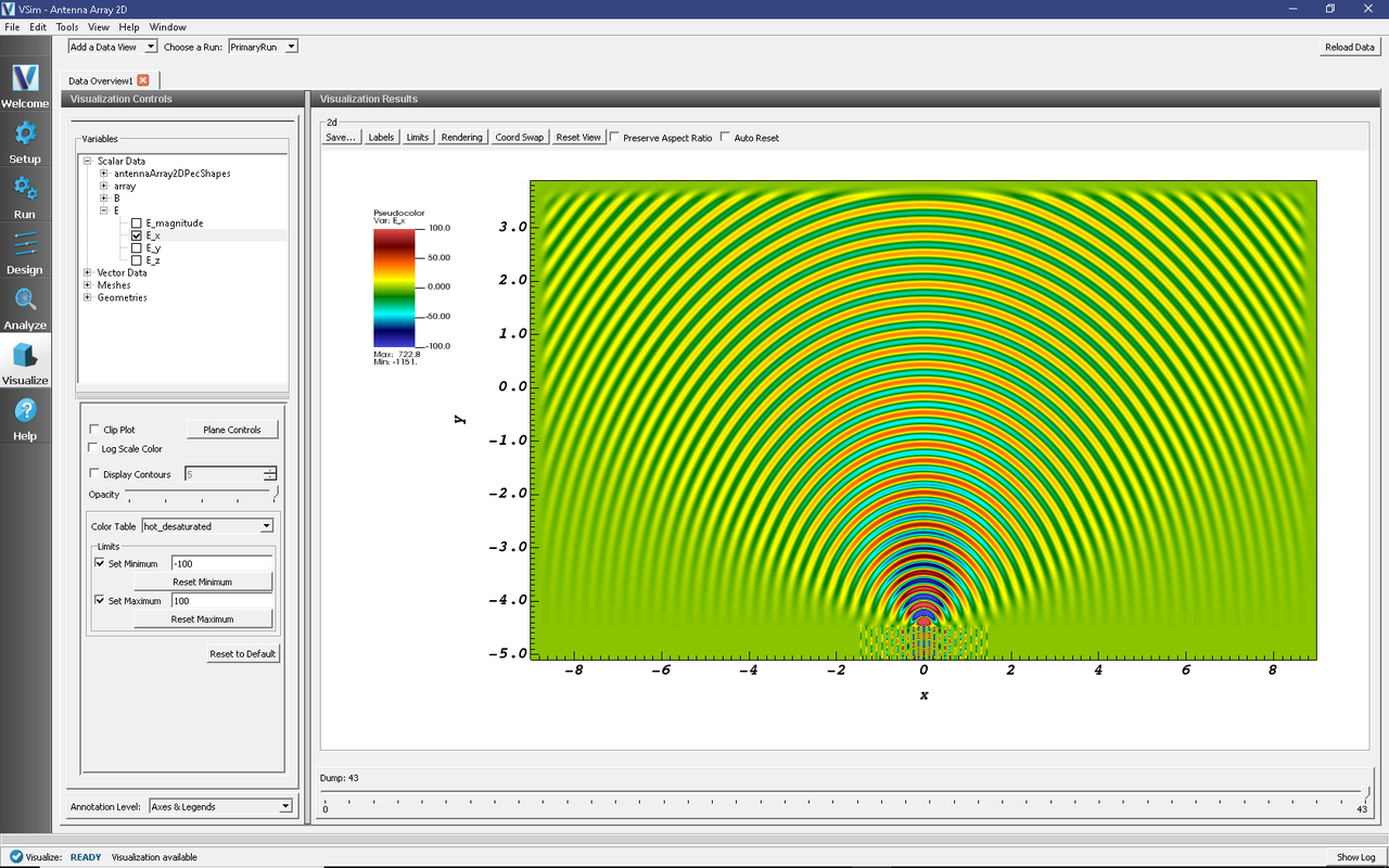
Fig. 191 The near and far electric fields in the x-direction at the end of the simulation.
Figure Fig. 191 shows the near and far electric fields at the end of the simulation run. The dispersion of the electric field through the non-excited waveguides can also be seen.
Single Element Antenna
Expand Constants
Change constants N_ELEM to 1
Change N_EXCITED_ELEM to 1
Expand Geometries
Expand CSG
Remove array
Remove gapArray
Select metal, hold Ctrl, select gap, right click → Boolean Operation → select metal_gap
Select metalMinusgap
For material select PEC from the drop-down menu
You can now assign any name of your choice to the metalMinusgap geometry (e.g., aperture). Save and proceed to the Run tab. Follow the same run steps as described above in the section Running the Simulation.
Second viz is shown in Fig. 192.
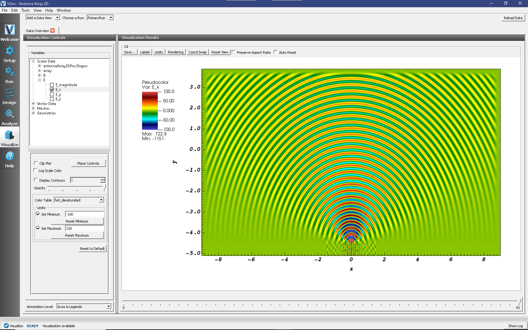
Fig. 192 The near and far electric fields in the x-direction for a 1-element antenna.
Calibration Runs
For both the multiple-element and single-element antenna simulations, calibration runs are needed for the analyzer.
For the original multiple-element array setup, proceed as follows:
Proceed to the Setup Window
In the top left corner, select File → Save Simulation As …
Rename the simulation to antennaArray2DCalibration.sdf
Note
If your simulation has a different name, add the word Calibration before .sdf
Click Save
Expand Geometries
Expand CSG
Remove array
Remove gapArray
Select gap
Change the height to HEIGHT_METAL_CALIB
Change the x position setting to XBGN_EXCITED_GAP
Select metal
Change the height to HEIGHT_METAL_CALIB
Click on metal, hold down Ctrl button and select gap right click → Boolean Operation
Select metal_gap
Select metalMinusgap
Select PEC under material from the drop-down menu.
You can now assign any name of your choice to the metalMinusgap geometry (e.g., myWaveguide).
Expand Field Dynamics
Expand FieldBoundaryConditions
Remove malUpperY
Right-click FieldBoundaryConditions → Add FIeldBoundaryCondition → select Port
Select upper y for the boundary surface from the drop-down menu
Save and proceed to the Run tab.
Change Number of Steps to 7800
Note
The calibration number of steps must equal the total number of steps that the simulation ran for during the regular run.
Repeat the same steps for the single-element antenna simulation setup.
Analyzing the Results
After performing the above actions, continue as follows:
Proceed to the Analysis Window by pressing the Analyze button in the navigation column.
Open the compute2DantennaGainAndPhase.py analyzer by selecting it and selecting “open”.
The default analyzer fields are the following:
simulationName: antennaArray2D
dumpNr: 30
nlambda: 15.0
gapWidth: 0.03
center: 0.0,-4.4969
dt: 5.59290428954e-12
freq: 1000000000.0
The overwrite box should be checked
Click Analyze in the top right corner.
The analysis is completed when you see the output shown in Fig. 193.
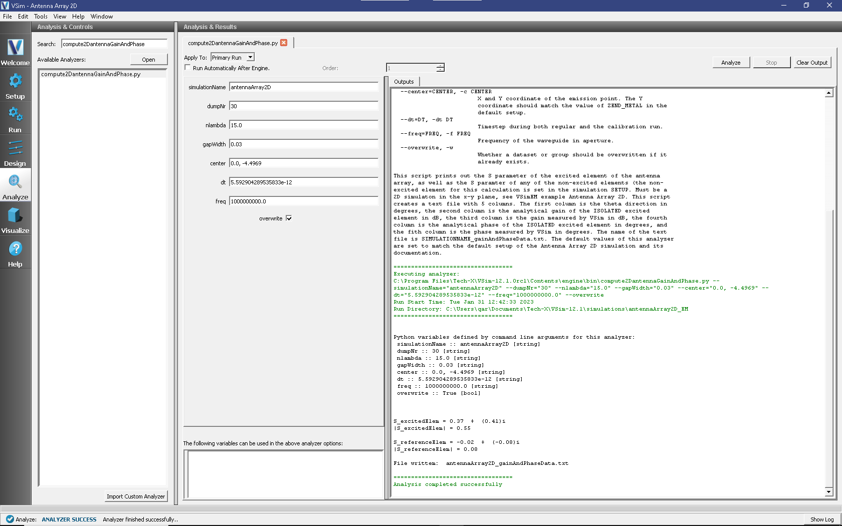
Fig. 193 The S-parameters for the excited element as well as the reference element associated with the constant S_PARAM_ELEM in the simulation setup are shown at the end of the analyzer run.
The S-parameters for the excited element as well as the reference element associated with the constant S_PARAM_ELEM in the simulation setup are shown at the end of the analyzer run.
This analyzer creates a text file with 5 columns. The first column is the theta direction in degrees, the second column is the analytical gain of the ISOLATED excited element in dB, the third column is the gain measured by VSim in dB, the fourth column is the analytical phase of the ISOLATED excited element in degrees, and the fith column is the phase measured by VSim in degrees. The name of the text file is SIMULATIONNAME_gainAndPhaseData.txt.
For the default simulation settings (i.e., the center element of a 25-element array is excited while the other elements are turned off), plotting the second and third columns (analytical and measured gains) against the first column (as a function of theta) will give the results shown in Fig. 194.
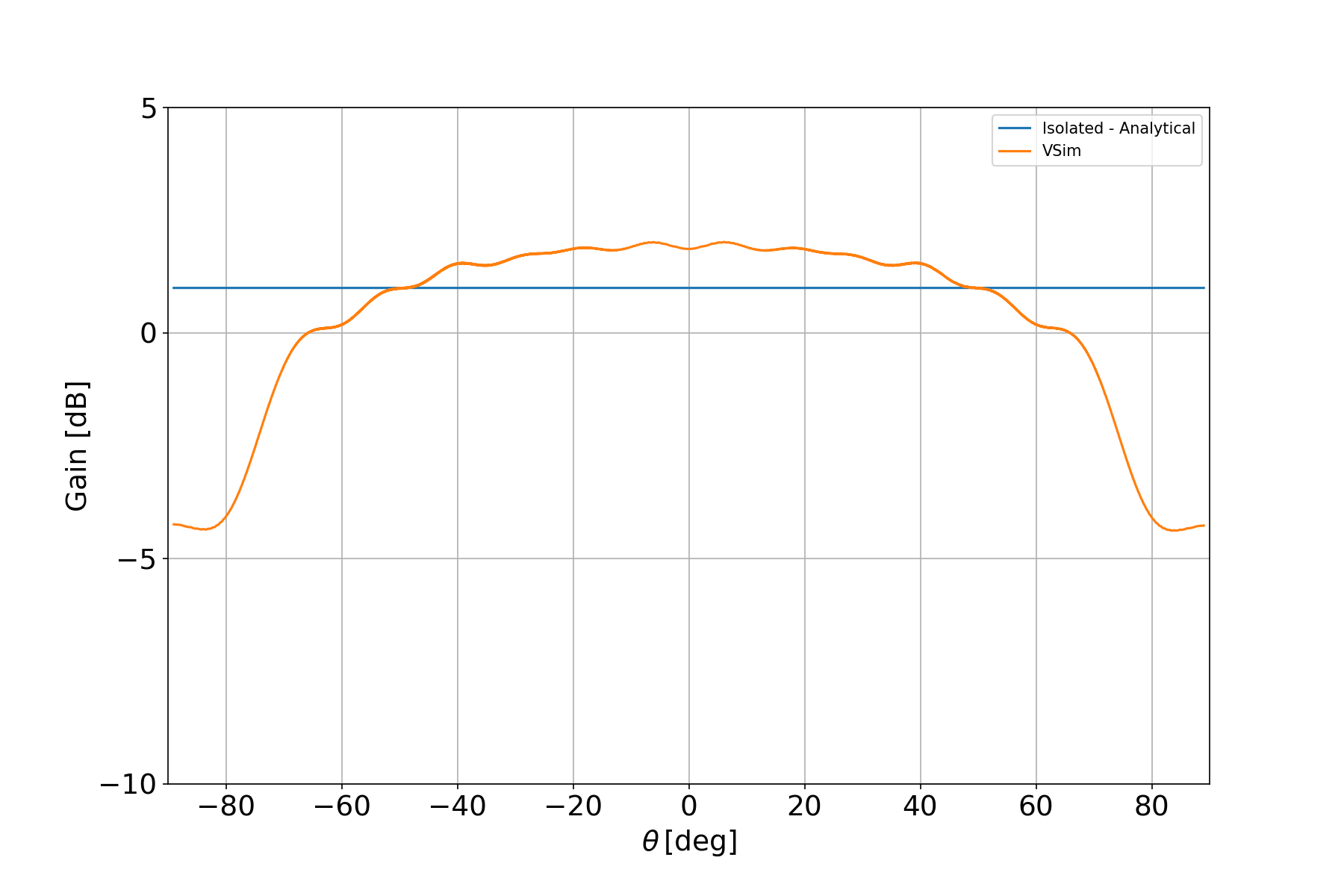
Fig. 194 The gain pattern of a 25-element array with the center excited element.
Plotting the fourth and third columns (analytical and measured field phases) against the first column (as a function of theta) will give the results shown in Fig. 195.
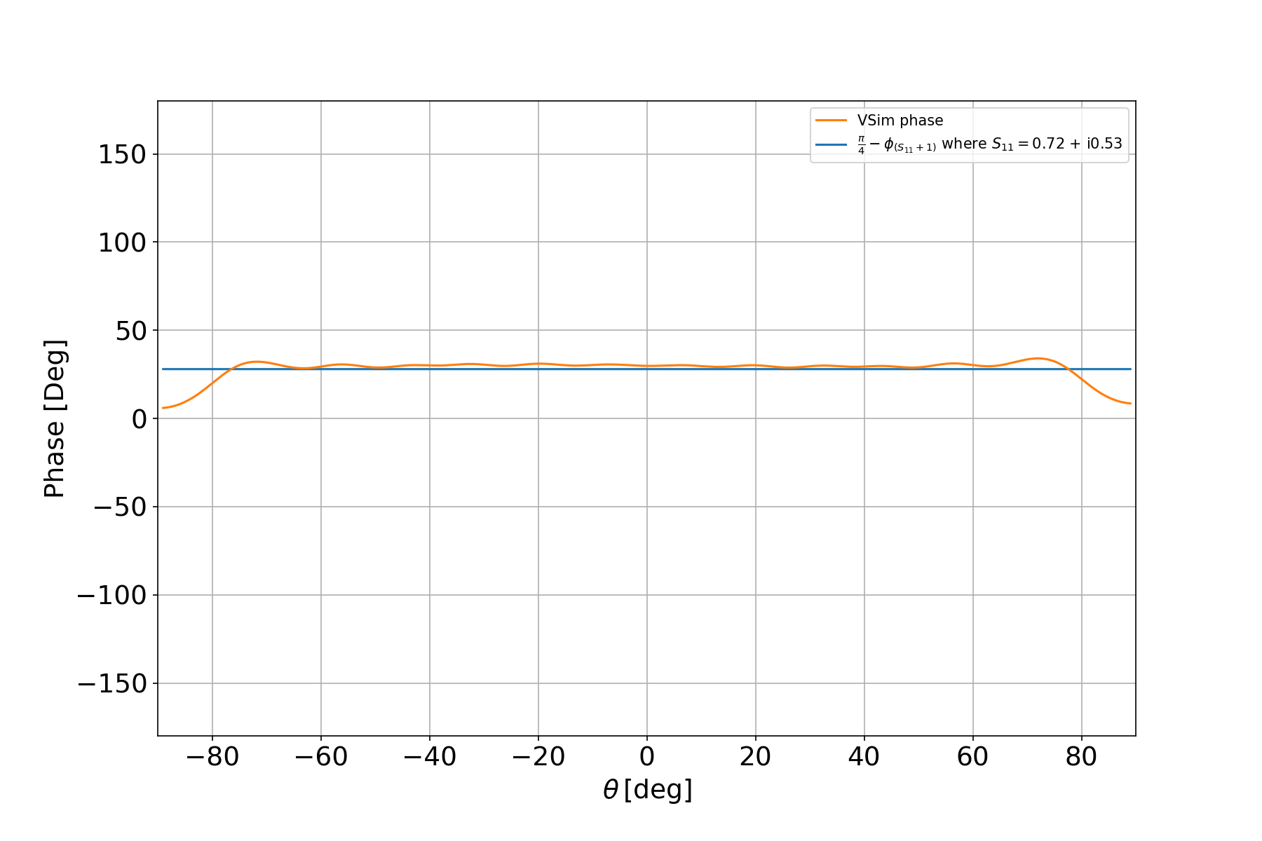
Fig. 195 The phase pattern of a 25-element array with the center excited element.
Further Experiments
A different array of geometries can be created changing input parameters such as number of elements in the array (N_ELEM) and the distance between the elements in each direction (DIST_ELEM). After changing these Constants, to create a different antenna array, proceed as follows:
Expand Geometries
Expand CSG
Right-click on gap → Create Array
In the Array Description window, select the “Union elements” checkbox, type in the number of elements to the value under N_ELEM, and the distance between elements to the value under DIST_ELEM. Then select the CSG “metal”, hold down Ctrl and select gapElemUnion located at the end of the gap array elements → Boolean Operation → select metal_gapElemUnion. Rename accordingly and assign the material PEC to the newly created geometry.
Repeating the analysis steps for a 1-element antenna (N_ELEM = 1 in the simulation setup) will give the results shown in Fig. 196 and Fig. 197.
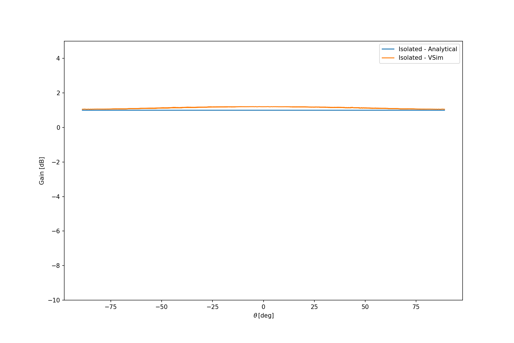
Fig. 196 The gain pattern of a 1-element array.
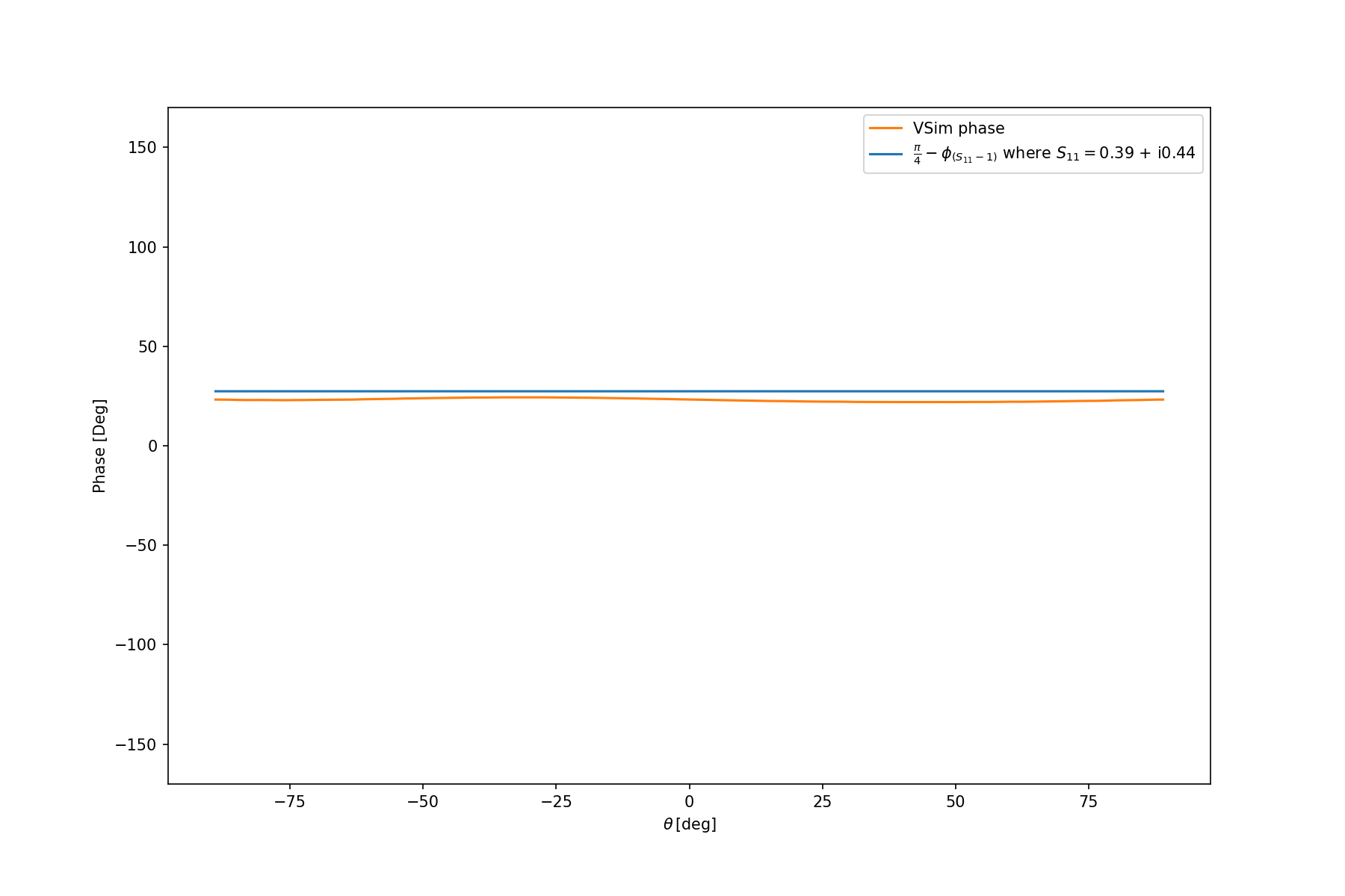
Fig. 197 The phase pattern of a 1-element array.
A different element can be excited by changing input parameter N_EXCITED_ELEM.
Repeating the analysis steps for a 25-element antenna with the edge element excited (N_EXCITED_ELEM = 25 in the simulation setup) will give the results shown in Fig. 198 and Fig. 199.
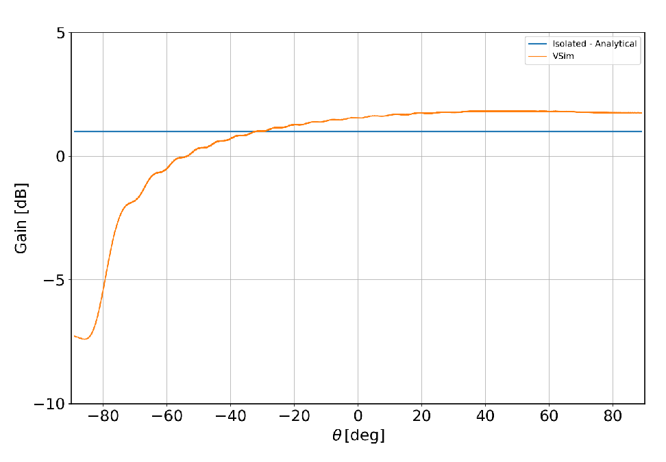
Fig. 198 The gain pattern of a 25-element array with the edge excited element.
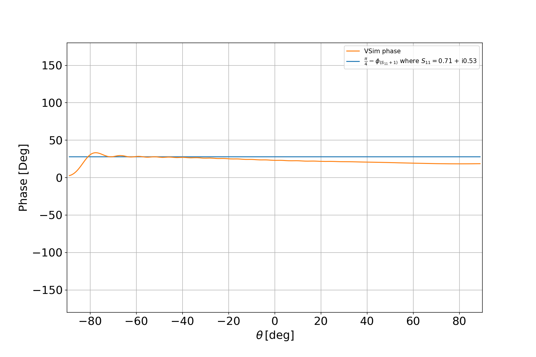
Fig. 199 The phase pattern of a 25-element array with the edge excited element.