Phased Array Antenna (phasedArrayAntenna.sdf)
Keywords:
- phasedArrayAntenna, far field, radiation
Problem Description
This VSimEM example illustrates how to setup a phased array simulation and analyze the far field results. Phased array antennas are a vastly-expanding field of research and development due to the fact that going from a one element antenna to an N-element antenna provides more directive beamforming characteristics and, most importantly, non-mechanical steering. Creating a multiple-element antenna results in an array pattern composed of wires, apertures, or other element types. Directive patterns are obtained via constructive interference in the desired direction and destructive in the other directions. Applications of phased array antennas range from commercial (5G, wireless & mobile, satellite telecommunication), military & defense (RADAR, acoustics) to research: atmospheric, space.
For a full walkthrough of this example see the video below: https://www.youtube.com/watch?v=5-I8dmHv8qU&list=PLottQ0Bg2M-3ATV5O9IP-3TEC4toVYPAK&index=12
This simulation can be run with a VSimEM license.
Opening the Simulation
The phasedArrayAntenna example is accessed from within VSimComposer by the following actions:
Select the New → From Example… menu item in the File menu.
In the resulting Examples window expand the VSim for Electromagnetics option.
Expand the Antennas option.
Select Phased Array and press the Choose button.
In the resulting dialog, create a New Folder if desired, then press the Save button to create a copy of this example.
The resulting Setup Window is shown Fig. 231.

Fig. 231 Setup Window for the Phased Array example.
Simulation Properties
This example consist of \(15\times 15\) array of small metal antenna elements excited by a distributed current source. The separation between the elements is \(\frac{\lambda}{6}\).
Note that the SPACING parameter CANNOT be used in the CSG array setup settings. To recreate an array with a different spacing between elements, the spacing needs to first be calculated and then typed into the array setup window.
The current source is results in an outging wave centered at \((x,y)=(0,0)\). The wave amplitude has a Gaussian profile with the standard deviation \(\sigma\). The phase and amplitude are tied to the azimuthal angle \(\theta\), and polar angle \(\phi\). In this example, the azimuthal angle \(\theta\) is fixed at \(\pi/4\) via the Function dphiFunc. The polar angle \(\phi\) goes from 0 to \(2\pi\) throughout the simulation via the Function thetaFunc.
The simulation domain contains a far field box history that is later used for the computeFarFieldFromKirchhoffBox analyser.
The current excitation formula, \(F(x, y, \phi, \theta, t)\), is:
Where the aplitude \(A(x,y,\phi,\theta)\), the phase \(\Phi(x,y,\phi,\theta)\), and locations in the x-y plane \(X(x)\) and \(Y(y)\) are defined by:
Running the Simulation
Once finished with the setup, continue as follows:
Proceed to the Run Window by pressing the Run button in the navigation column out left.
To run the file, click on the Run button in the upper left corner of the Logs and Output Files pane. You will see the output of the run in that pane. The run has completed successfully when you see the output, “Engine completed successfully.” This is shown in Fig. 232.
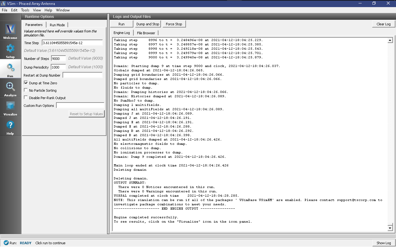
Fig. 232 The Run Window at the end of execution.
Analyzing the Results
After performing the above actions continue as follows to compute the far field radiation pattern:
Proceed to the Analysis Window by pressing the Analyze button in the navigation column.
In the resulting list, select computeFarFieldFromKirchhoffBox and press Open
The analyzer fields should be filled as below:
simulationName: phasedArrayAntenna
fieldLabel: E
farFieldRadius: 30.0
numPeriods: 0.25
numFarFieldTimes: 2
frequency: 1.0e9
numTheta: 16
numPhi: 32
zeroThetaDirection: (0,0,1)
zeroPhiDirection: (1,0,0)
incidentWaveAmplitude - blank
incidentWaveDirection - (0,0,0)
varyingMeshMaxRadius - 30.0
principalPlanesOnly - checked
Click Analyze in the top right corner.
The analysis is completed when you see the output shown in Fig. 233.
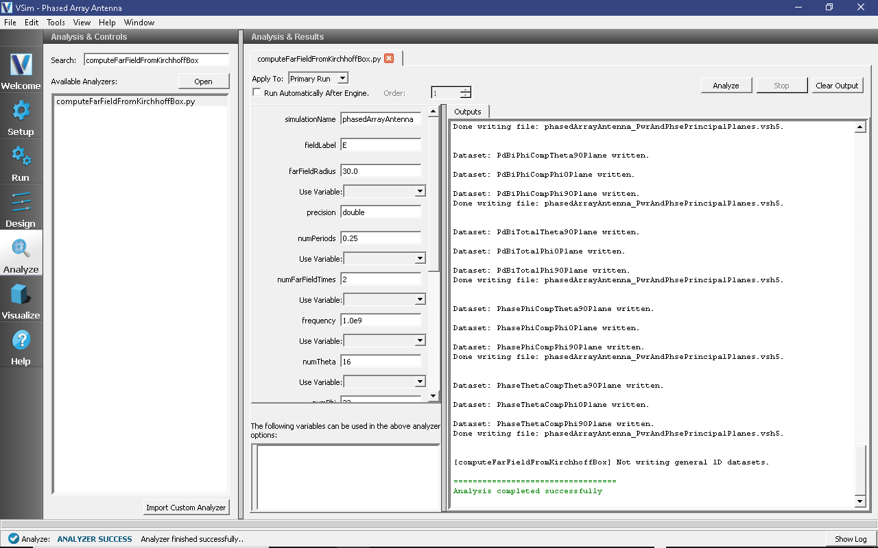
Fig. 233 The computeFarFieldFromKirchhoffBox at the end of a successful run.
For more accurate results, use the following input paramters in the analyzer:
simulationName: phasedArrayAntenna
fieldLabel: E
farFieldRadius: 30
numPeriods: 0.25
numFarFieldTimes: 2
frequency: 1e9
numTheta: 60
numPhi: 120
zeroThetaDirection: (0,0,1)
zeroPhiDirection: (1,0,0)
varyingRadiusMesh: 30.0
Visualizing the Results
After performing the above actions, the results can be visualized as follows:
Proceed to the Visualize Window by pressing the Visualize button in the navigation column.
From the Data View dropdown menu, select Data Overview.
Expand Scalar Data variables.
Expand farE and check the farE_Magnitude box.
Move the dump slider to see the evolution of the far fields in time.
The resulting visualization is shown in Fig. 234.
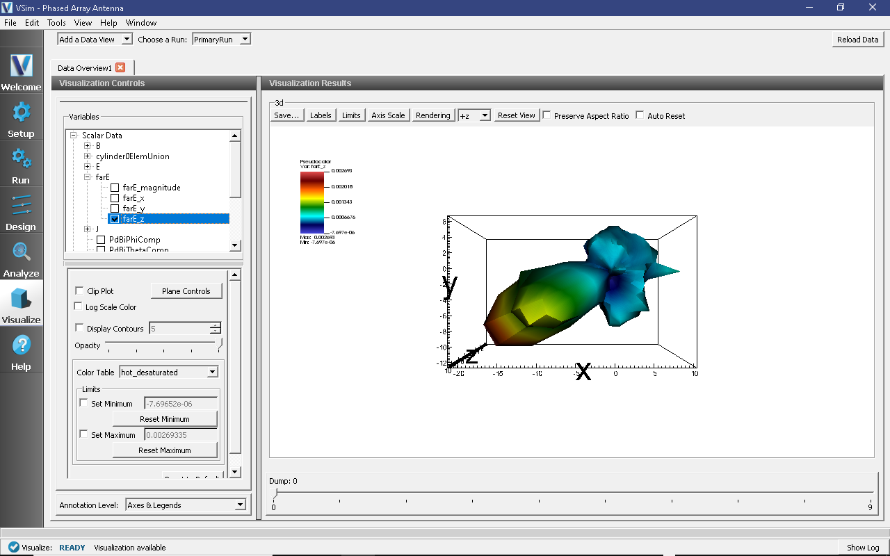
Fig. 234 Far field pattern 30 m away from the antenna.
To visualize the 2D far fields proceed as follows:
Proceed to the Visualize Window by pressing the Visualize button in the navigation column.
From the Data View dropdown menu, select Field Analysis
Under Field choose farE_magnitude
Move the dump slider to see the evolution of the 3D far fields as well as the 2D cross-sections in time.
The resulting visualization is shown in Fig. 235.
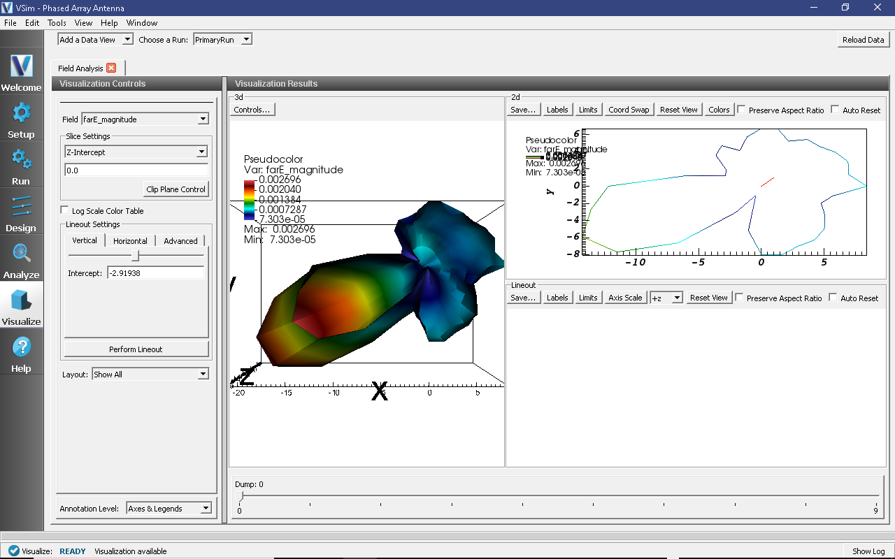
Fig. 235 2D cross-section of the far field patern measured 30 m away from the source.
This method of visualizing the far fields can be used for studying properties such as directivity, main and side lobe pattern, radiation strength, etc.