Half-Wave Dipole in Free Space (halfWaveDipoleAntenna.sdf)
Keywords:
- halfWaveDipoleAntenna, far field, radiation
Problem Description
This problem illustrates how to obtain far field radiation patterns from VSim simulation data. The simulation itself consists of a half-wavelength long current source in free space.
This simulation can be performed with a VSimEM license.
Opening the Simulation
The Half Wave Dipole Antenna example is accessed from within VSimComposer by the following actions:
Select the New → From Example… menu item in the File menu.
In the resulting Examples window expand the VSim for Electromagnetics option.
Expand the Antennas option.
Select “Half-Wave Dipole in Free Space” and press the Choose button.
In the resulting dialog, create a New Folder if desired, and press the Save button to create a copy of this example.
All of the properties and values that create the simulation are now
available in the Setup Window as shown in
Fig. 218. You can expand the tree
elements and navigate through the various properties, making any
changes you desire. The right pane shows a 3D view of the geometry, if
any, as well as the grid, if actively shown. To show or hide the grid,
expand the Grid element and select or deselect the box next to
Grid.
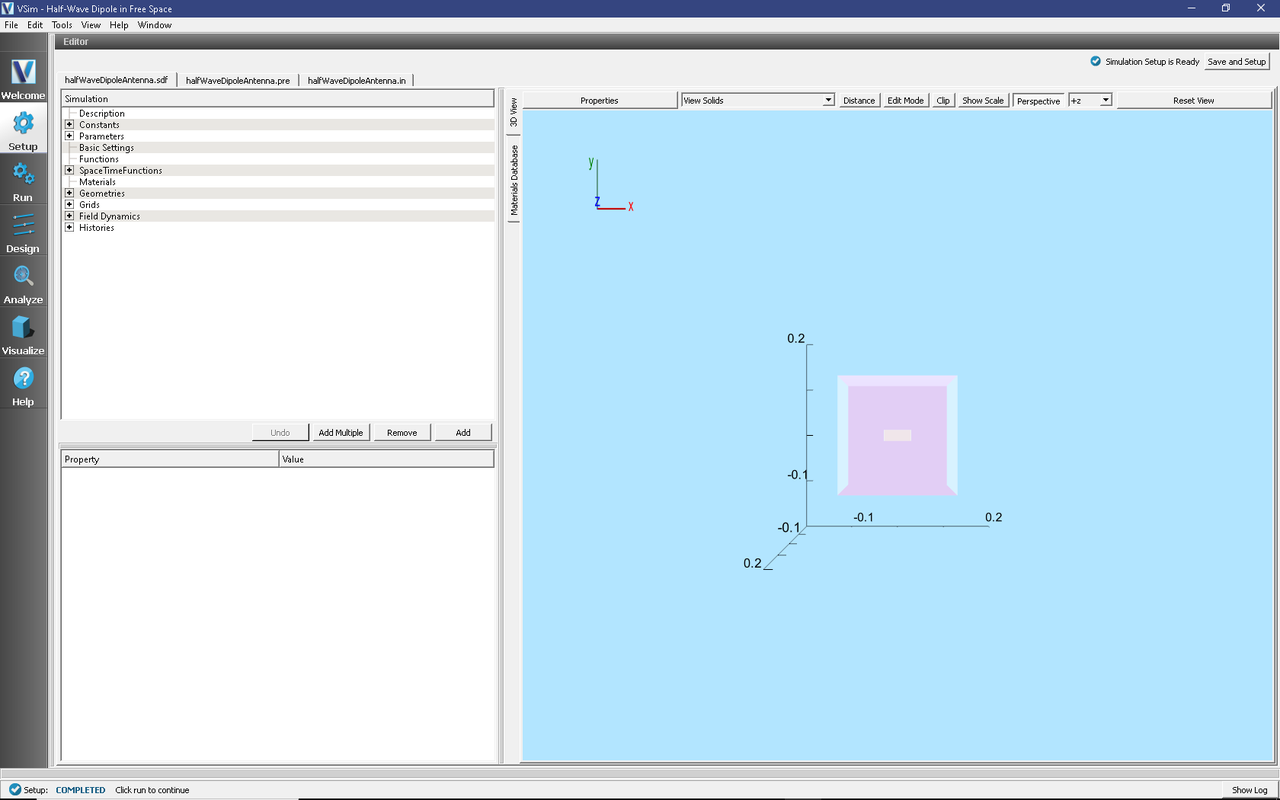
Fig. 218 Setup Window for the Half Wave Dipole Antenna example.
Simulation Properties
This example includes Constants for easy adjustment of simulation properties, Including:
AMPLITUDE: The amplitude of the signal
FREQUENCY: The frequency of the antenna
There are also SpaceTimeFunctions to define the current driver of the half wavelength source.
Other properties of the simulation include open boundaries on all sides. A Distributed Current source is used to set the current of the half wavelength antenna.
Running the Simulation
After performing the above actions, continue as follows:
Proceed to the run window by pressing the Run button in the left column of buttons.
To run the file, click on the Run button in the upper left corner of the right panel. You will see the output of the run in the right pane. The run has completed when you see the output, “Engine completed successfully.” This is shown in Fig. 219.
NOTE: the correct elements will not appear in the visualization step if the analysis step has not been performed first.
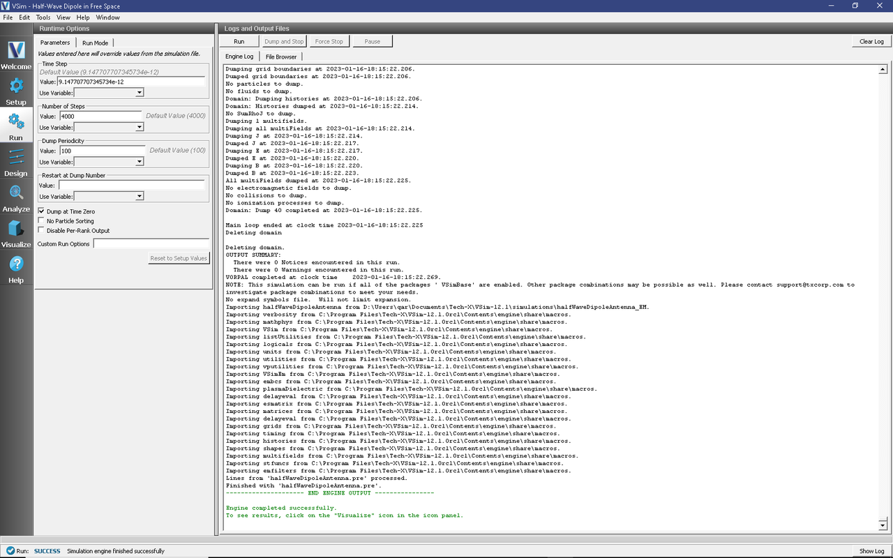
Fig. 219 The Run Window at the end of execution.
Analyzing the Results
After performing the above actions, continue as follows:
Proceed to the Analysis window by pressing the Analyze button in the left column of buttons.
Select computeFarFieldFromKirchhoffBox.py (default). Then click Open.
For this example, edit the following input parameters:
simulationName - halfWaveDipoleAntenna (name of the input file)
fieldLabel - E (name of the electromagnetic field)
farFieldRadius - 10.0 (radius of the far sphere, i.e., distance to the far zone)
numPeriods - 0.25
numFarFieldTimes - 2
frequency - 3.0e9
numTheta - 45 (number of points in the theta direction)
numPhi - 90 (number of points in the phi direction)
zeroThetaDirection - (0,0,1) (determines orientation of far field coordinate system)
zeroPhiDirection - (1,0,0) (determines orientation of far field coordinate system
incidentWaveAmplitude - blank
incidentWaveDirection - (0,0,0)
varyingMeshMaxRadius - 10.0
principalPlanesOnly - checked
Click the Analyze button in the upper right corner.
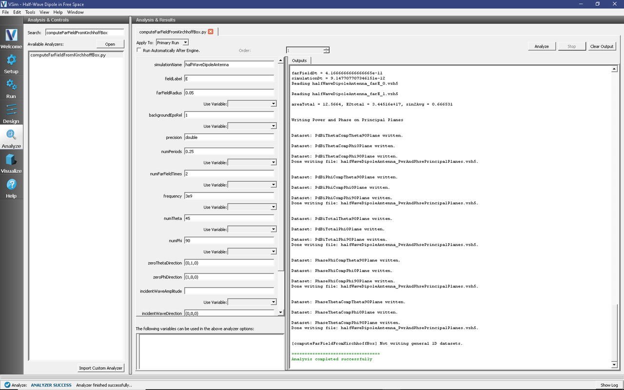
Fig. 220 The Analysis window at the end of execution.
Visualizing the Results
After performing the above actions, continue as follows:
Proceed to the Visualize Window by pressing the Visualize button in the left column of buttons.
The far field radiation pattern can be found in the scalar data variables of the data overview tab:
Expand Scalar Data
Expand farE
Select farE_magnitude
Move the dump slider forward in time to see the evolution
Click and drag to rotate the image
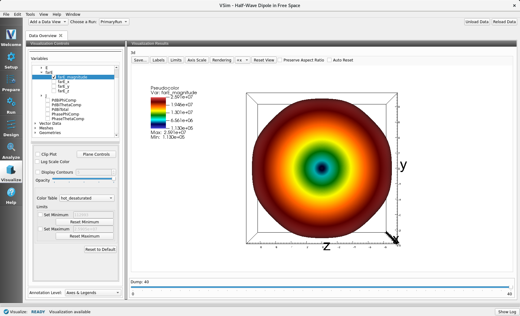
Fig. 221 The far field radiation pattern
Further Experiments
The resolution of the far field pattern can be changed by editing the number of theta, phi, and sphere points in the far field history.
Try implementing a conducting plane to see how it affects the far field.
If the Simulation domain is made too small, the results will be distorted as the entire near field must be within the simulation domain in order to achieve a proper transformation to the far field.