Magnetic Fields of Wire (bFieldByJT.pre)
Keywords:
- Calculating A vector by a current-carrying long linear wire.
Problem description
This simulation illustrates how to model magnetostatics. A straight current, Jo, is directed along the z-axis. The example solves Poisson’s equation for the vector potential, A. The 0th dump of the simulation is the analytical solution for the purpose of comparison.
This simulation can be performed with a VSimBase license.
Opening the Simulation
The magnetic field by a current example is accessed from within VSimComposer by the following actions:
Select the New → From Example… menu item in the File menu.
In the resulting Examples window expand the VSim for Basic Physics option.
Expand the Basic Examples (text-based setup) option.
Select “Magnetic Fields of Wire (text-based setup)” and press the Choose button.
In the resulting dialog, create a New Folder if desired, and press the Save button to create a copy of this example.
The basic variables of this problem should now be alterable via the text boxes in the left pane of the Setup Window, as shown in Fig. 181.
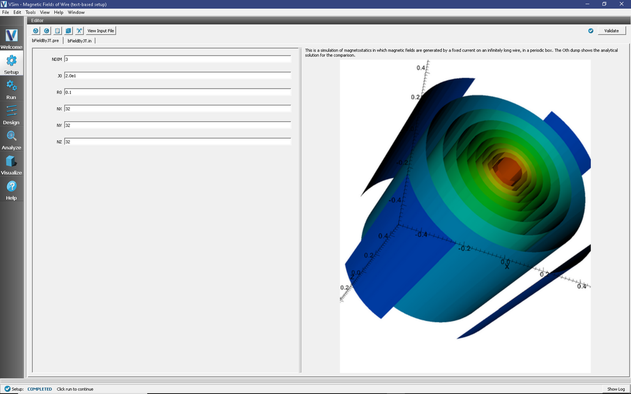
Fig. 181 Setup Window for the magnetic field by a current.
Input File Features
VSimComposer allows the user to vary the applied current and a radius of the wire. These are the main parameters that affect the A vector. By changing these parameters, a user can run simulations to explore how the A vector depends on the applied current and radius. The input file, when viewed in the editor, also exposes all the grid sizes of the simulation that are used by the implemented models.
Running the simulation
After performing the above actions, continue as follows:
Proceed to the Run Window by pressing the Run button in the left column of buttons.
To run the file, click on the Run button in the upper left corner of the Logs and Output Files pane. You will see the output of the run in the right pane. The run has completed when you see the output, “Engine completed successfully.” This is shown in Fig. 182.
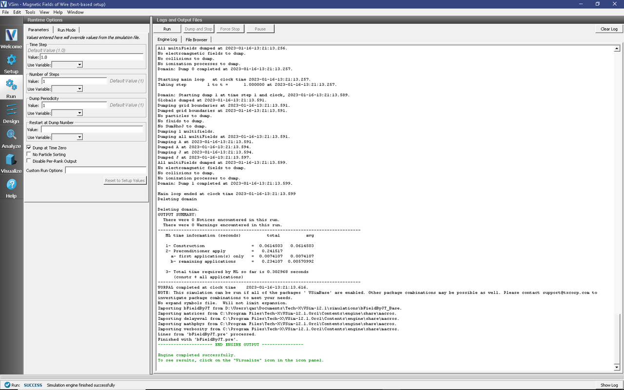
Fig. 182 The Run Window at the end of execution.
Visualizing the results
After performing the above actions, continue as follows:
Proceed to the Visualize Window by pressing the Visualize button in the left column of buttons.
For this example, one can see the A vector fields. To see the A vector, continue as follows:
Make sure the Data View drop down is set to Data Overview.
Here you can see Variables. Expand the Scalar Data. Then expand A
Four variables are available, the three components of A and the magnitude of the vector. Select A_magnitude.
Check the box next to Display Contours
Rotate the view by clicking and dragging your mouse.
Fig. 183 shows the visualization seen for A_magnitude.
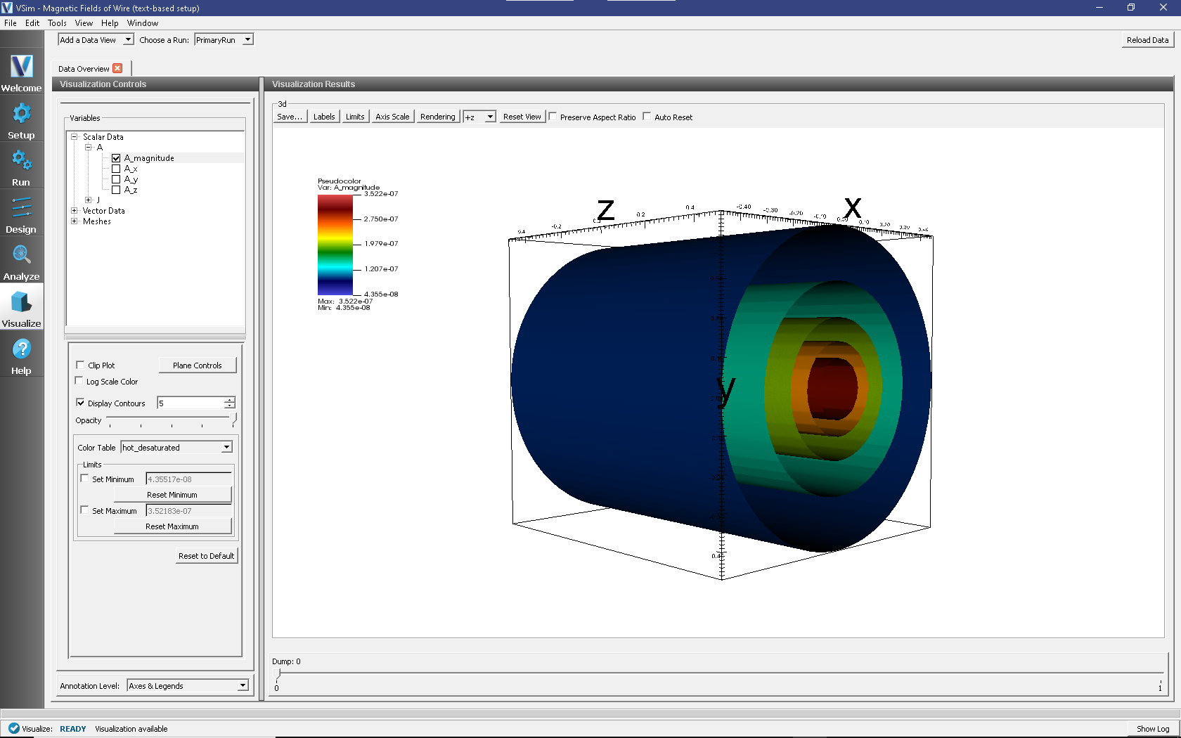
Fig. 183 Visualization of magnetic fields by the current as a color contour plot.
Further Experiments
This input file can be modified to test different current, and wire radius. This will allow users to study how to use the magnetostatics capability in Vorpal.