Dipole Radiation (dipole.sdf)

Problem Description

An oscillating electric dipole is one of the the simplest radiation sources. The dipole moment oscillates with a given frequency which then results in electromagnetic radiation being emitted at the same frequency. The electromagnetic field may be calculated for distances from the source that may be comparable to the wavelength, or distances far away from the source, in the so-called radiation zone. The radiated power is not distributed isotropically, but assumes the shape of a toroid. The Poynting vector averaged over a complete cycle is given by

Where \(p_0\) is the dipole moment, \(\omega\) is the angular frequency. In the set up, an ideal dipole of zero length is located at the center of the computational domain and pointing along the y axis. The oscillation of the dipole is gradually turned on, with a given rise time. The radiation that exits the computational domain gets absorbed into MAL layers. The fields produced by the radiation may be computed within the computational domain, or for points far away from the source that lie beyond the compuational domain. This is done with the help of an analyzer that is part of the VSim distribution. The histories of the electric and magnetic fields are recorded along a closed surface known as a Kirchoff box that lies within the MAL layers. This field information is then used to compute fields at points far away from the radiation source by applying the Kirchoff integral theorem.

The current set up has a frequency for 0.3 GHz, resulting in a wavelength of about 1m. The grid refinement is set to 16 cells per wavelength, and the time step is chosen to be very close to the Courant condition. The computational domain extends to 1.5 times the wavelength along either side of the origin along each coordinate axis. The MAL thickness is 2 wavelengths thick which covers the computational domain.

This simulation can be run with a VSimEM, VSimMD, or VSimPD license.

Opening the Simulation

The Dipole Far Field example is accessed from within VSimComposer by the following actions:

• Select the New → From Example… menu item in the File menu.
• In the resulting Examples window expand the VSim for Electromagnetics option.
• Expand the AntennasT option.
• Select Dipole Far Field and press the Choose button.
• In the resulting dialog box, create a New Folder if desired, then press the Save button to create a copy of this example.

The resulting Setup Window is shown in Fig. 219.

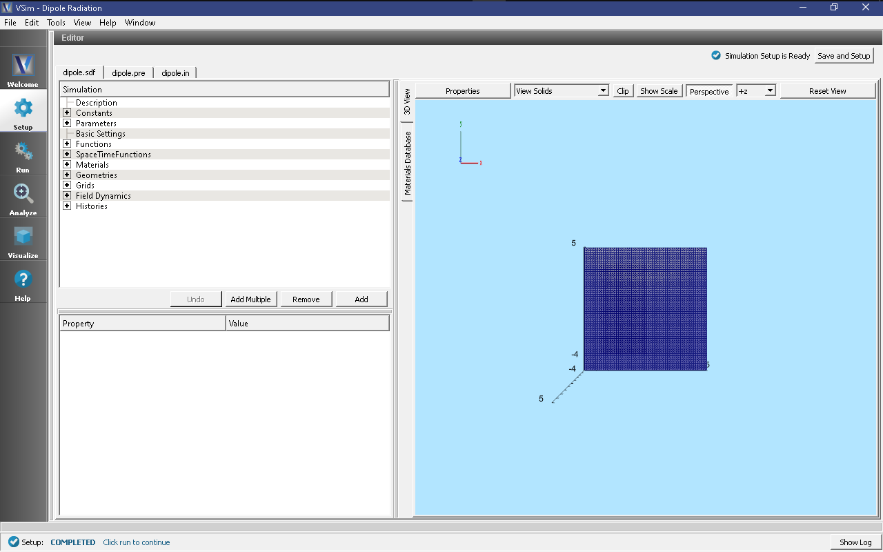
Fig. 219 Setup Window for the Dipole example.

Running the Simulation

To run the simulation:

• Proceed to the run window by pressing the Run button in the left column of buttons.
• Here you can set run parameters, including how many cores to run with (under the MPI tab).
• When you are finished setting run parameters, click on the Run button in the upper left corner. You will see the output of the run in the right pane.

The run has completed when you see the output, “Engine completed successfully.” This is shown in Fig. 220. The number of steps chosen in this run is sufficient so that the radiation reaches the Kirchoff box and the field histories are recorded for a sufficient duration.

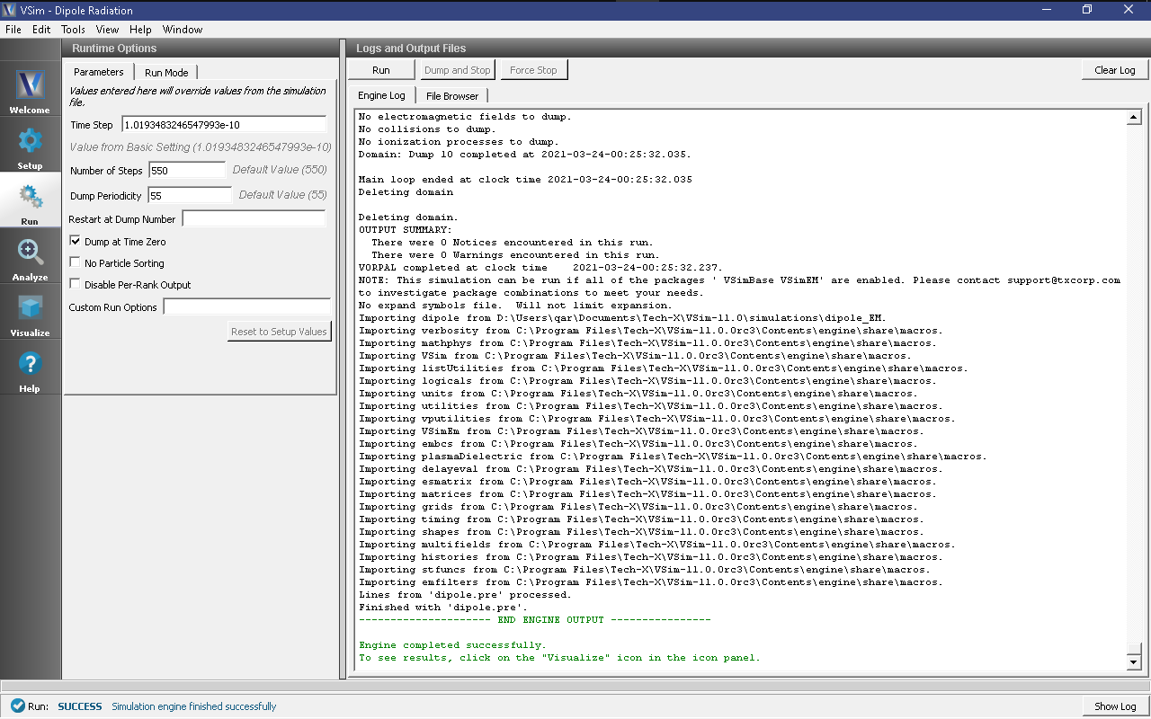
Fig. 220 The Run window at the end of execution.

Running the Analyzer

After completing the run, one can run the analyzer to compute field values at far away points. To bring up the analyser script, Click on the Analyze icon. The panel that appears will be named computeFarFieldFromKirchoffBox.py, along with a set of text boxes in which the necessary parameters need to be filled. For the defailt settings of the file you may use the following:

• simulationName - dipole
• fieldLabel - E
• farFieldRadius - 1024.0
• numPeriods - 0.25
• numFarFieldTimes - 2
• frequency - 0.3e9
• numTheta - 17
• numPhi - 17
• zeroThetaDirection - (0,1,0)
• zeroPhiDirection - (0,0,1)
• incidentWaveAmplitude - blank
• incidentWaveDirection - (0,0,0)
• varyingMeshMaxRadius - 1024.0
• principalPlanesOnly - checked

Note that some entries need to be left blank. After entering the above parameters, also shown in Fig. 221, press the “Analyse” button that appears on the upper right side.

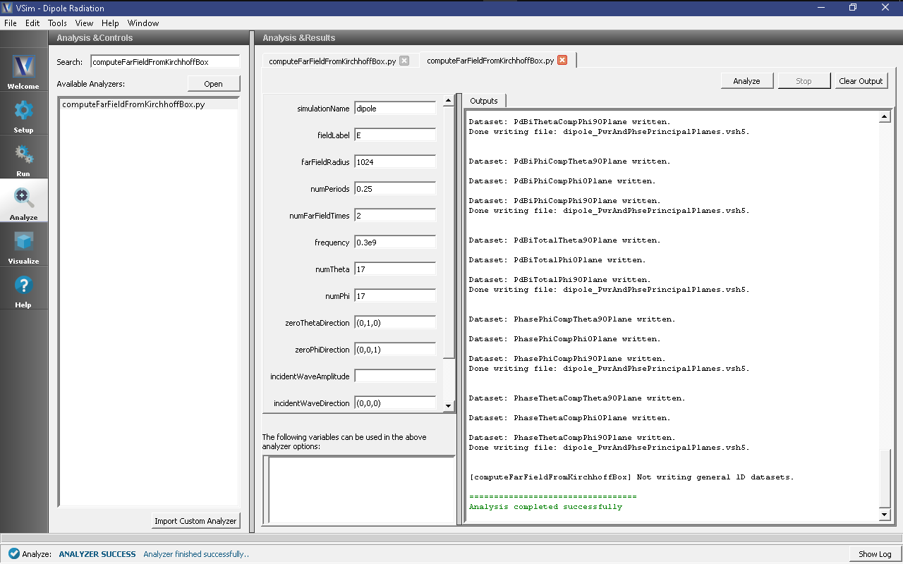
Fig. 221 The Analyze Window at the end of analyzer execution.

Visualizing the Results

After performing the above actions, the results can be visualized as follows:

1. Proceed to the Visualize Window by pressing the Visualize button in the navigation column.
2. With the Add a Data View expanded, click on Field Analysis.
3. In the Visulaization Controls section, expand the Field menu and click on farE_magnitude.
4. Choose X-Intercept in the Slice settings, and choose 3d Only in Layout.

Use the mouse to orient the torus as shown in Fig. 222.

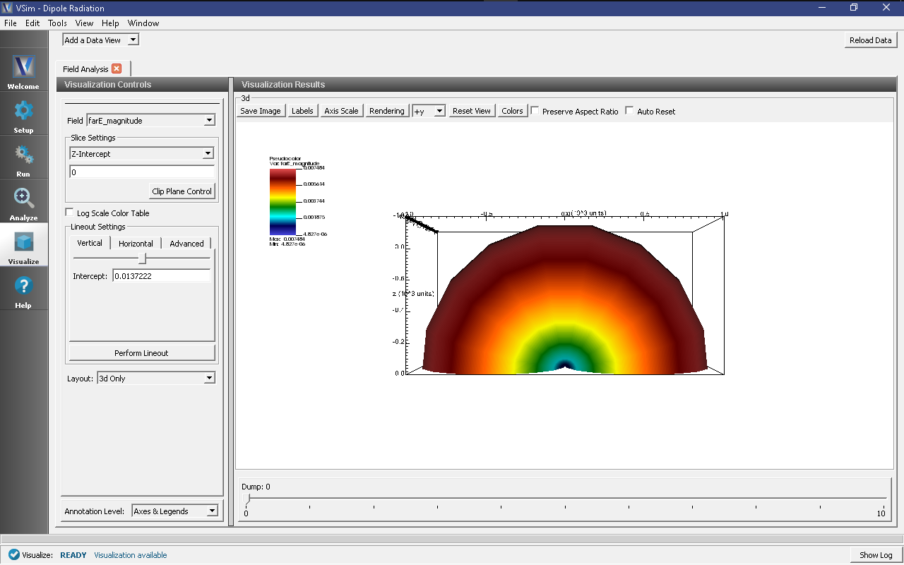
Fig. 222 The magnitude of the electric field is propotional to the time averaged power flux.

Choosing Parameters Within the Far Field Box

It is important that the simulation is run for long enough so that sufficient data is logged in the histories, which is necessary to perform the Kirchhoff box analysis. Most examples involve a rise-time when the amplitude of the wave is gradually ramped up. After this, an EM wave with a steady amplitude begins to propagate. It is necessary that recording of the data on the Kirchhoff box surface begins after the rise-time, or once the steady stay amplitude sets in. Another factor to be noted is the time taken for the wave, travelling at the speed of light, to reach the Kirchoff box surface from the source. This time period depends on the location of the source. In the dipole radiation source example, it is at the center of the similation domain, while in some other examples, the wave may be launched from one end of the simulation domain. The duration of observation, or logging of the histories data, must be the sum of the following two quantities, (1) at least 2.5 wave periods (2) time taken for the wave to transit between opposite corners of the Kirchhoff box. The outer surface of the Kirchhoff box needs to lie within the region that is bounded by the inner surface of MAL layer. The perpendicular distance between the outer surface of the Kirchhoff box and the nearest inner surface of the MAL layer may be about 3 cells.

In the set up window, click on the Histories drop down menu. Following this, click on farFieldBox0 and then on measurement. One can toggle between choosing the start and end of measurement in units of time or time-steps, as shown in Fig. 223.

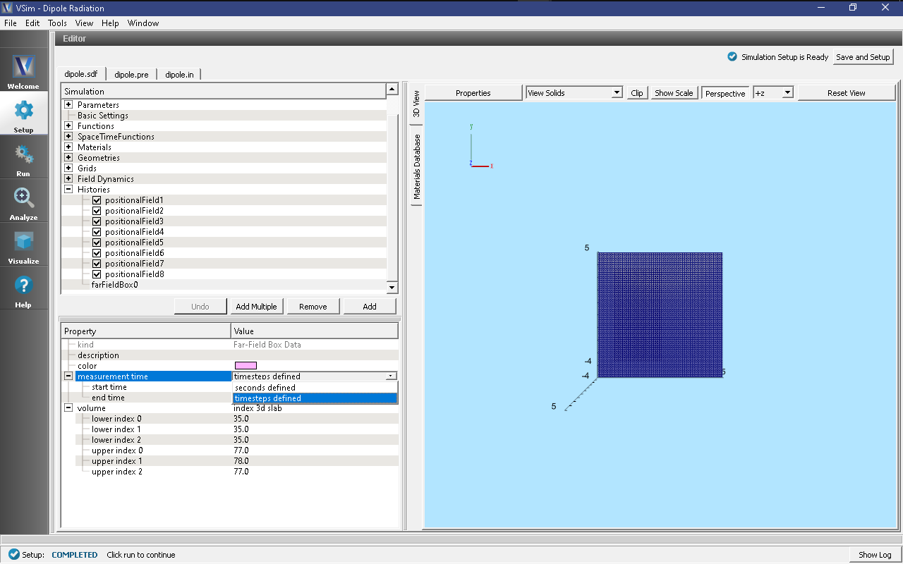
Fig. 223 Setting the FarField box parameters

The start parameter must be specified, in the appropriate units as,

where, an arbitrary user specified observe start time has been added, which the user can set to any value equal to or greater than zero. The domain transit time is the time taken for the wave to travel from one corner to the opposite corner of the Kirchhoff box. The end parameter must then be specified, in the appropriate units as,

As already mentioned, observe periods needs to be equivalent to 2.5 wave periods.

The results of the simulation are not affected if the total period of observation exceeds the minimum requirement. The above set of parameters result in an observation time that is sufficiently large when applied to any example in this document that involves using the Kirchhoff box.

Further Experiments

Change some of the parameters such as frequency or dipole moment in the set up window to see a variation in the radiated power.