Overview of Using Analyzers

Using An Example To Demostrate How to Use an Analyzer

First we open an example and run a simulation in order to get some data to analyze. Open the two stream example and follow along:

• Select the New -> From Example menu item in the File menu.
• In the resulting Examples window, expand the VSim for Basic Physics option.
• Expand the Basic Examples option.
• Select Two-Stream Instability and press the Choose button.
• In the resulting dialog, create a new folder if desired, and press the Save button to create a copy of this example in your run area.
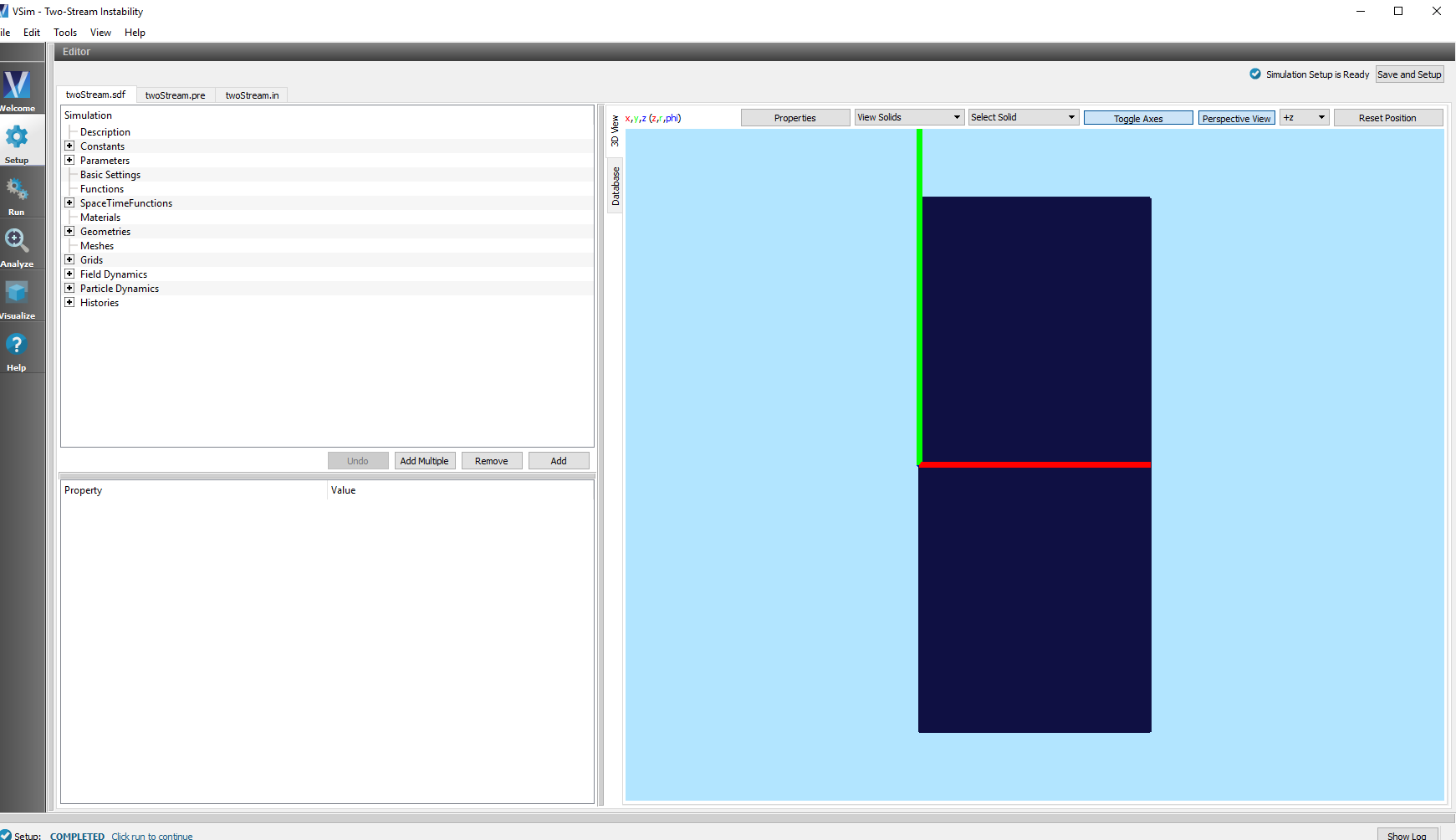
• This will open the Two-Stream Instabilitiy example. For this exercise, we will use the default parameters.

See Fig. 97.

Fig. 97 Setup Window for Two Stream Example

Select an Analyzer (Installed with VSim)

VSimComposer allows the user to select a analzer from the Analyze window. You can type in the name of an analyzer to filter and shorten the list or double-click any analyzer in the list. You can also select the Import Analyzer button at the bottom to import your own customized script.

For the two stream example, wait until the simulation run has completed and then click on the Analyze tab located below the Run tab on the left hand side of the screen.

• In the Analysis Controls pane, a list of all of the analyzers will be available.
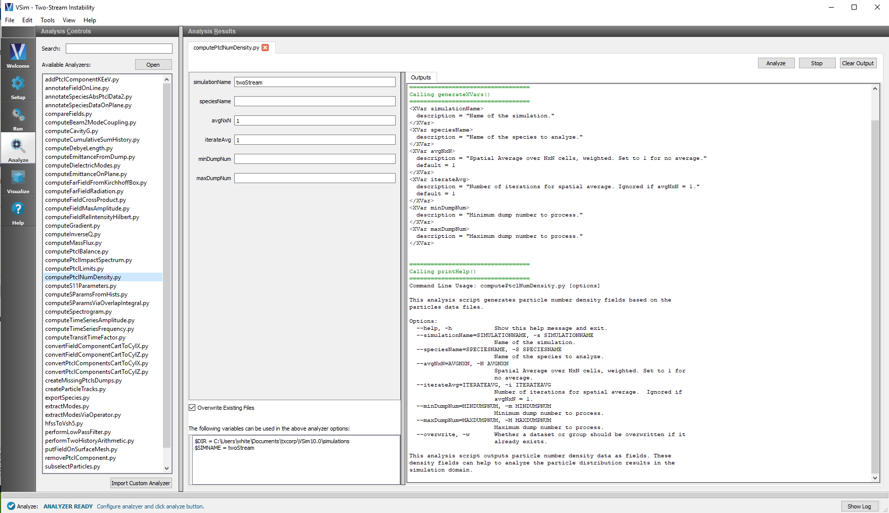
• For this example, we will select computePtclNumDensity.py.
• In the Analysis Results pane and under the Outputs tab, instructions as to which variables have to be given by the user will appear.
• For this particular analyzer, the only two variables are the simulationName and the speciesName. For simulationName, give it the name of the simulation, in our case twoStream. The speciesName parameter is either electrons0 or electrons1, the two species of electrons in this simulation.

See Fig. 98.

Fig. 98 Analysis Window with Parameters

This process should be the same for both visual and text-based simulations.

However, there are different processes for keeping analyzers available for your simulation through closing and reopening. For visual setup, simply run your simulation and analyzer of choice as usual, and then return to the Setup tab and select the Save and Setup button in the top right. This process saves your analyzer in the .sdf file for your simulation.

Running the Analyzer

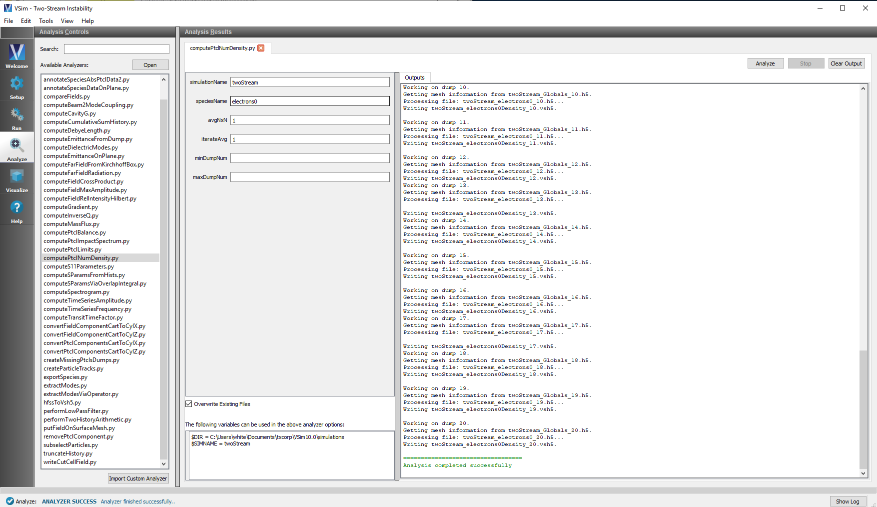
Click the Analyze button located at the top right of the Control pane.

Fig. 99 Analysis Window Successful Run

Output of an Analyzer

The data generated from the execution of an analyzer will be stored as a .vsh5 file and is visualizable underneath the Visualize tab. Be aware that the analyzer may also produce data that it writes to the screen or as hdf5 output.

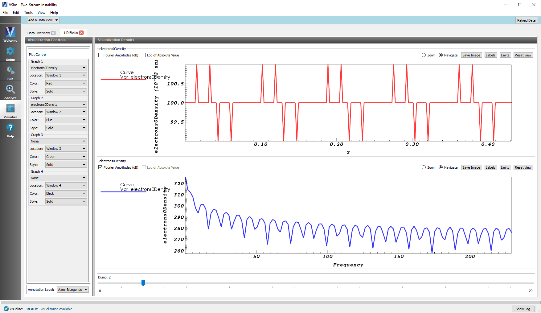
Finishing up with the two stream example, the data we got from computePtclNumDensity.py can be visualized through the following:

• Open the Visualize tab. You may need to click on the Reload Data button at the top right of the Visualization Controls pane if you have gone back and forth between the windows and the VSim computational engine has generated more data.
• Switch the Data View drop-down menu at the top left of the pane to 1-D Fields.
• For Graph 1, select electrons0Density for the Base Variable from the drop-down menu under Graph 1.
• For Graph 2, select electrons0Density again for the Base Variable. In the Visualization Results pane (2nd graph), click the Fourier Amplitudes box to see the Fast Fourier Transform output of the frequency domain.
• To match the visualization of this documentation, select Dump 2 in the slide bar at the bottom of the Visualization Results pane.

You can explore other visualization options in this window, or can rerun the simulation with different parameters to investigate further.

Fig. 100 Visualization of the analysis data