Grids
The grids used by VSim are structured, coordinate aligned, where the grid lines are along coordinate directions. Such a two-dimensional grid is shown in Fig. 34. One can choose either a uniform spacing or a non-uniform spacing as shown in Fig. 34, and the coordinates may be either cartesian or cylindrical. In Fig. 34, each of the cells is numbered by its indices. In this \(2D\) case, there are two indices; in general one for each direction. The cell indices start at \(0\) and end in the \(x\) direction at \(NX - 1\) for a grid that has \(NX\) cells in the \(x\) direction. For a \(3D\) grid, there would be another direction out of the page.
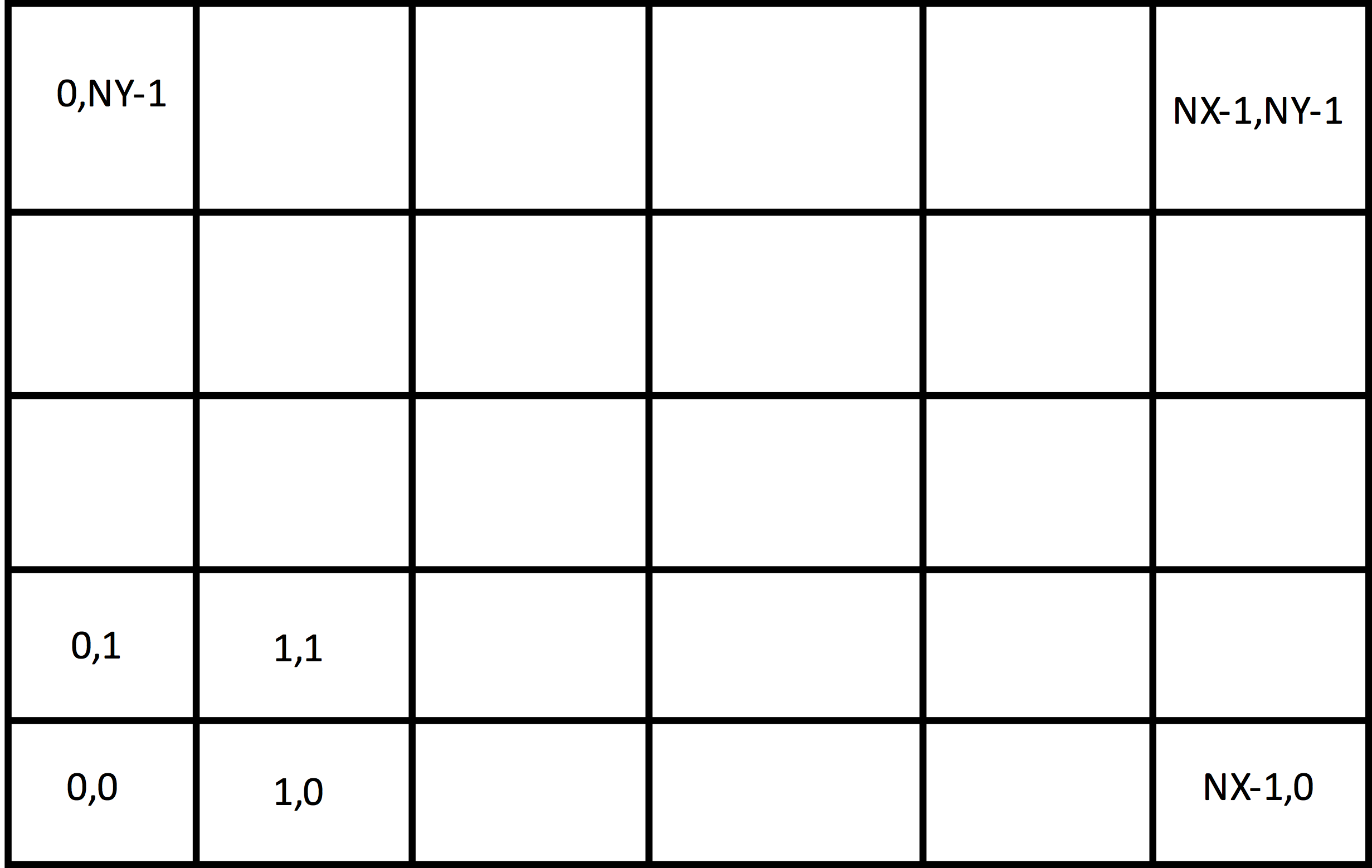
Fig. 34 Structured 2D grid.
A cell of a 3D grid is shown with z coming out of the page in two views in Fig. 35. A cell owns its interior plus the interior of its lower face in each direction plus, the interior of its lower edge in each direction, plus the lower node of its owned edges. The owned node is circled in both views of Fig. 35. The owned edges are shown on the left side of Fig. 35, with the x-edge red, the y-edge green, and the z-edge blue. Similarly, the owned faces of a cell are shown on the right side of Fig. 35, with the x-normal face red, the y-normal face green, and the z-normal face blue.
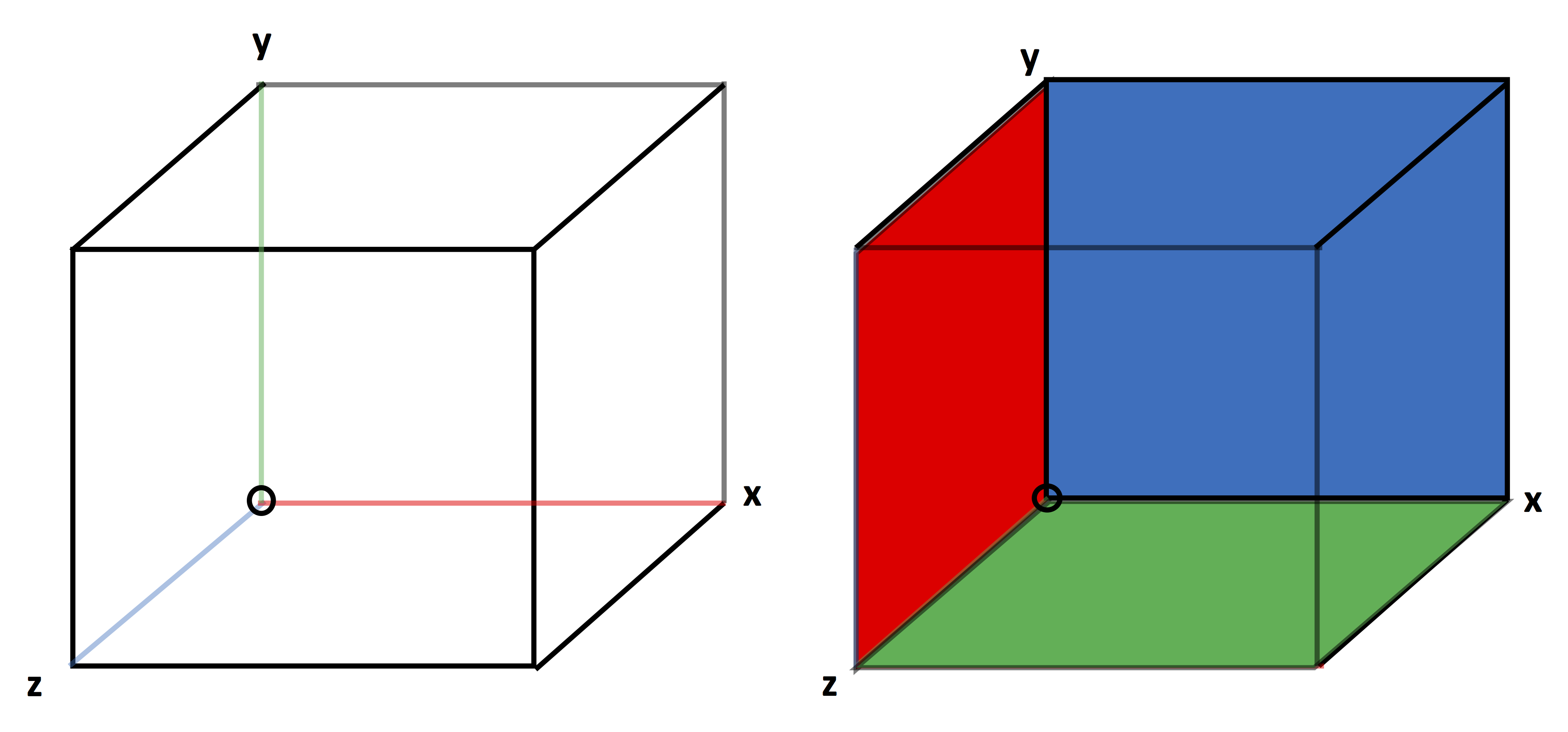
Fig. 35 3D cell in a view showing its edges and a view showing its faces.
In FDTD EM, the concept of a dual grid is useful. The dual grid is the grid with nodes at the centers of the regular grid. The edges of the dual grid pierce the faces of the regular grid and vice-versa.
Guard cells
Guard cells, cells just outside the simulation grid, are needed for having sufficient field values in the simulation region, for particle boundary conditions, and for parallel communication (to be dicussed later). An example of the first case is where a field must be know at each of the nodes of the simulation. Then, since the last node in any direction is owned by the cell one beyond the simulation, the cells one beyond the physical grid must be in the simulation. Thus, the grid must be extended by one cell in the last of each direction, as shown in Fig. 36.
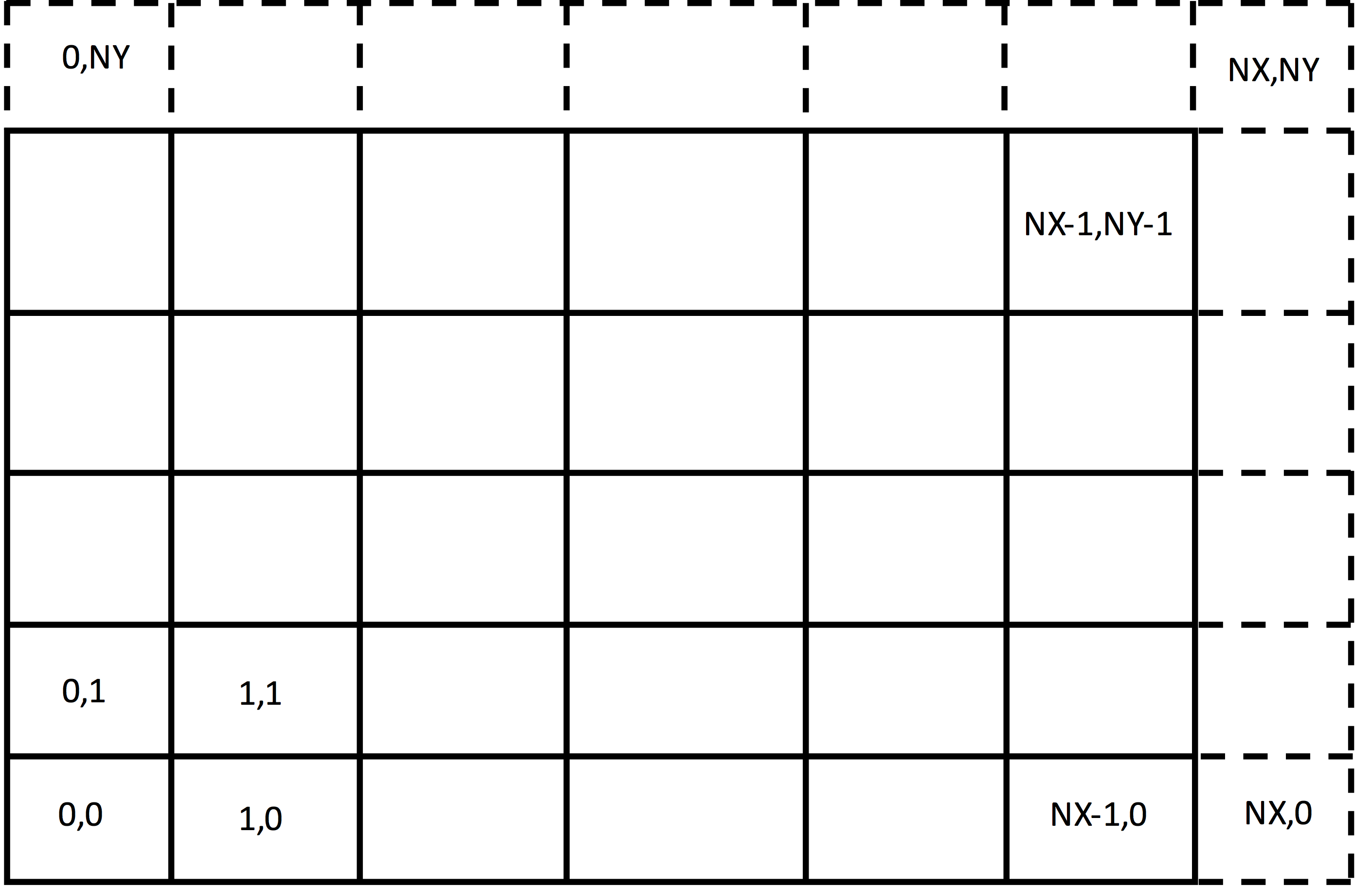
Fig. 36 Grid extended to include the upper nodes, which belong to the cells one past the last cell in each direction.
Note
The user-defined grid is called the physical domain. The grid extended by Vorpal is called the extended domain.
For particle boundary conditions, the grid must be further extended down by one cell in each direction. When a particle leaves the physical domain, it can end up in one of these additional cells, which can be either above or below. A data value associated with that cell determines what to do with the particle, e.g., absorb it (remove it), reflect it, or carry out some other process. The associated extended grid is shown in Fig. 37. The physical cells are depicted by the red grid. The associated dimensions are in blue. The extended cells (shown in green) enclose both the physical cells and the guard cells added by Vorpal.
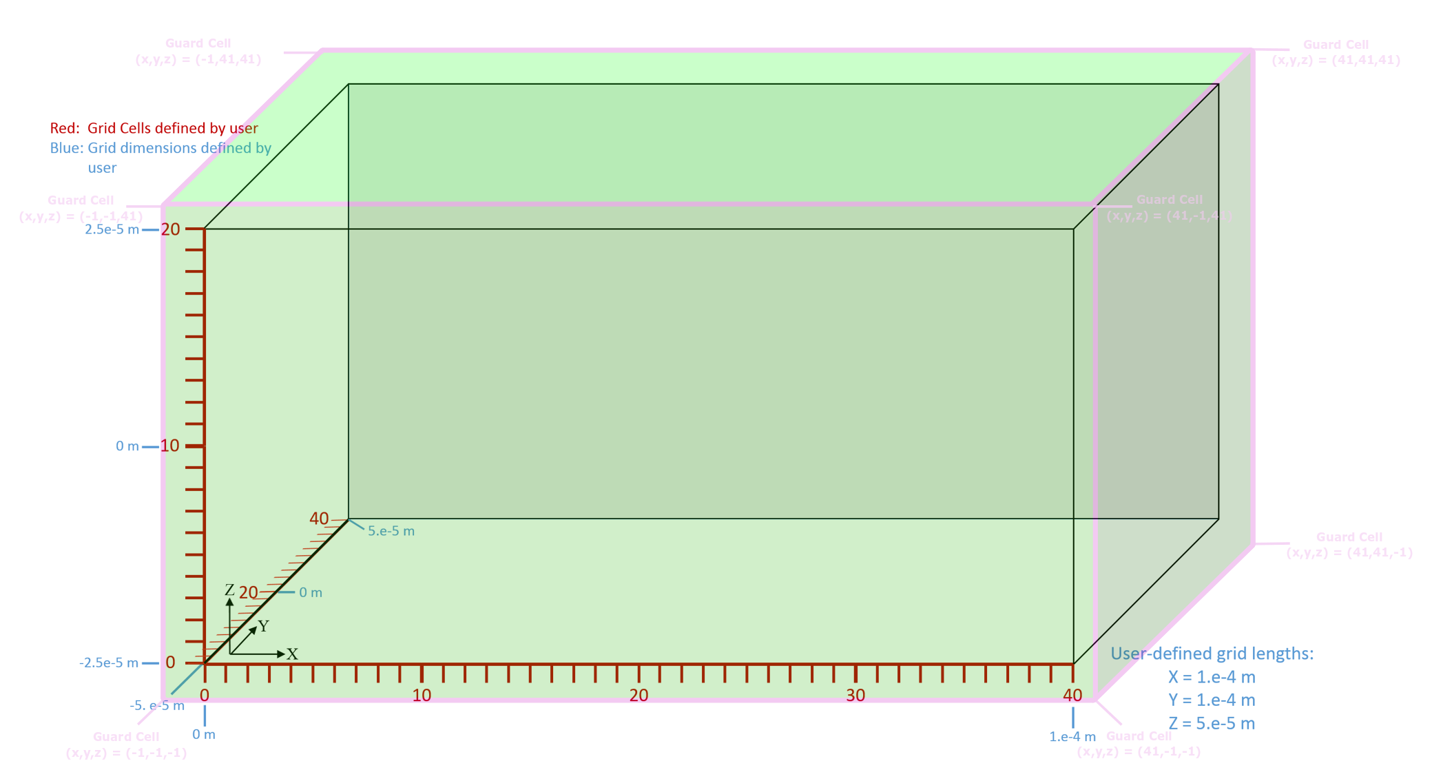
Fig. 37 Cartesian grid extended by Vorpal
Periodic Boundary Conditions
Periodic boundary conditions can be used to control both field and particle behavior at the edge of the simulation domain. In the case of particles, periodic boundaries ensure that particles leaving one side of the domain reappear at the opposite side. For example, particles traveling at a speed of \(-v_{\phi}\) will go through \(\phi = 0\) and reappear at \(\phi = 2\pi\). Fields, on the other hand, will be copied from the plane at index \(0\) to the plane at \(NX\) and from the plane at \(NX-1\) to the plane at \(-1\), i.e. from the last physical cell to the guard cell on the other side.
Parallelism and Decomposition
Parallel (distributed memory, MPI) computation is carried out by domain decomposition. A particular decomposition is shown in Fig. 38. In this case, this is a decomposition of a rectangular region by the red lines, with the individual subdomains each give a unique index. However, Vorpal can simulate any region that is a non-overlapping collection of rectangles (appropriately generalized for 3D and 1D), with each rectangle being a subdomain of the decomposition.
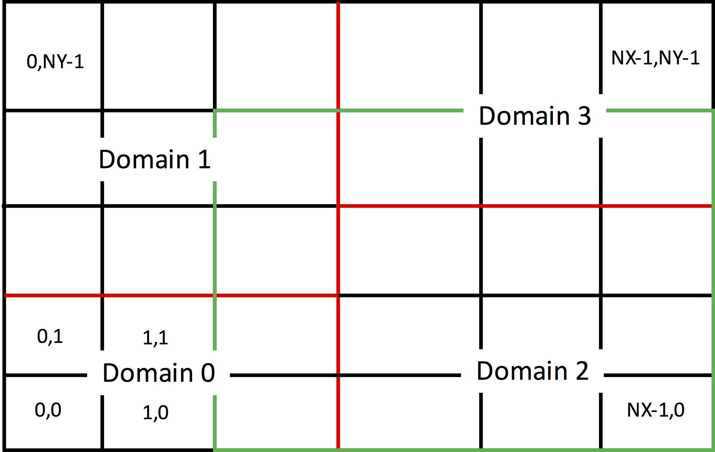
Fig. 38 Parallel decomposition of a computational domain.
For the most part, parallelism and decomposition are handled under the hood, but it is useful to understand a few concepts. In Fig. 38 one can see a green rectangle that extends one cell more into the simulation region beyond Domain 2. Fields in the cells of this overlap region are computed by the subdomain holding the cell, but they have to be communicated to Domain 2, as it needs this boundary region to update its fields on the next time step. On the other hand, particles may leave Domain 2 and end up in one of the cells still inside the green rectangle. Those particles must be sent to the processor holding the cell they are in for further computation.
For the above situation to work, the field update method for a given cell must not need information more than one cell away. The standard updates for electromagnetics and fluids indeed have this property. As well, the particles must not travel more than one cell in a time step. This is true for explicit electromagnetic PIC with relativistic particles, as the Courant condition prevents the time step from being larger than the time it takes for light to cross any cell dimension, and relativistic particles travel slower than the speed of light. Finally, the particles must not interpolate from fields more than one cell cell away, nor must they deposit current more than one cell away. This is true for the simplest interpolation and deposition methods.
However, if you have electrostatic particles that travel more
than one cell per timestep, or particles that have a larger
deposition footprint, then manual setting of some parameters may
be necessary. In particular, the grid parameter,
maxCellXings, states the maximum number of cells a
particle might cross in a simulation, and the parameter,
maxIntDepHalfWidth, provides the width of the deposition
stencil. From these follow the overlap needed for the
subdomains. These parameters are discussed in more detail later.