Two-Stream Instability (twoStream.sdf)
Keywords:
- electromagnetics, two-stream instability
Problem Description
The two-stream instability is a rapidly growing collisionless plasma instability arising from small charge imbalances. A local imbalance leads to the acceleration or deceleration of particles in its vicinity, which in turn leads to an even stronger imbalance. One setup that allows one to easily observe the instability is two counter-streaming beams of identical charge in a periodic system. The advantage of this configuration is that the generated plasma wave becomes a standing wave, thus allowing us to easily observe the formation of the phase space vortices.
In this example, we use two electron streams. At \(t=0\) the streams have drift velocities of magnitude \(7.78 \times 10^6\) m/s. In order to accelerate the onset of the instability, the two particle beams are given a small sinusoidal perturbation in velocity space.
This simulation can be performed with a VSimBase license.
Opening the Simulation
The Two-Stream Instability example is accessed from within VSimComposer by the following actions:
Select the New → From Example… menu item in the File menu.
In the resulting Examples window expand the VSim for Basic Physics option.
Expand the Basic Examples option.
Select Two-Stream Instability and press the Choose button.
In the resulting dialog, create a New Folder if desired, and press the Save button to create a copy of this example.
All of the properties and values that create the simulation are now available in the Setup Window as shown in Fig. 178. You can expand the tree elements and navigate through the various properties, making any changes you desire. The right pane shows a 3D view of the geometry, if any, as well as the grid, if actively shown. To show or hide the grid, expand the Grid element and select or deselect the box next to Grid.
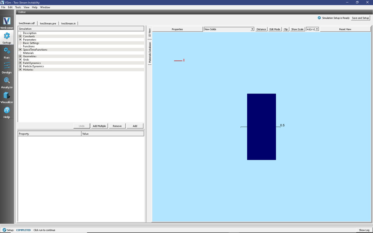
Fig. 178 Setup Window for the Two-Stream Instability example.
Simulation Properties
There are a number of Constants in this simulation to help make modifying the simulation even easier. Those include:
XCELLS: The number of cells
NOM_DEN_E: The electron density
VBAR: The average velocity
WAVELENGTHS: The number of wavelengths in the domain to simulate
PPC: The number of particles per cell.
SpaceTimeFunctions are used to set the velocities of each particle stream.
The simulation is 1 dimensional and periodic in x.
Running the Simulation
After performing the above actions, continue as follows:
Proceed to the Run Window by pressing the Run button in the left column of buttons.
To run the file, click on the Run button in the upper left corner of the window. You will see the output of the run in the right pane. The run has completed when you see the output, “Engine completed successfully.” This is shown in Fig. 179.
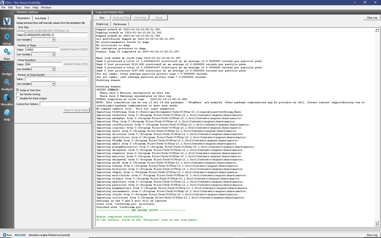
Fig. 179 The Run Window at the end of execution.
Visualizing the Results
After performing the above actions, continue as follows:
Proceed to the Visualize Window by pressing the Visualize button in the left column of buttons.
To view the instability as shown in Fig. 180, do the following:
Select the Phase Space option from the Data View menu
In the Plot 1 box, change the X-axis to electrons0_x, and the Y-axis to electrons0_ux
Click the Enable Second Plot box
In the Plot 2 box, change the Base Variable to electrons1, the X-axis to electrons1_x, and the Y-axis to electrons1_ux
Click the DRAW button at the bottom, then move the Dump slider forward in time.
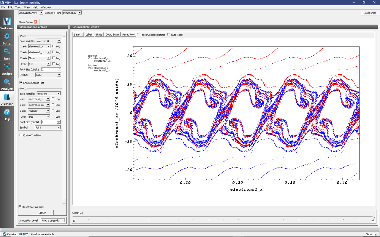
Fig. 180 Visualization of the two-stream instability developing in particle phase space.
Further Experiments
Change the average velocity and velocity modulation and see how the speed at which the instability sets in depends on the modulation.
View the particle density by using the computePtclNumDensity script in the Analyze Window.