Electromagnetic Plane Wave (emPlaneWave.sdf)
Keywords:
- electromagnetics, plane wave, periodic boundary conditions, wave launcher
Problem Description
A linearly-polarized (with electric field in the z-direction) continuous electromagnetic plane wave with a sinusoidal amplitude is launched from the left side (x=0) to propagate in the x-direction. The transverse (y,z) boundary conditions are periodic.
This simulation can be performed with a VSimBase license.
Opening the Simulation
The Electromagnetic Plane Wave example is accessed from within VSimComposer by the following actions:
Select the New → From Example… menu item in the File menu.
In the resulting Examples window expand the VSim for Basic Physics option.
Expand the Basic Examples option.
Select Electromagnetic Plane Wave and press the Choose button.
In the resulting dialog, create a New Folder if desired, and press the Save button to create a copy of this example.
All of the properties and values that create the simulation are now available
in the Setup Window as shown in Fig. 157.
You can expand the tree elements and navigate through the
various properties, making any changes you desire. The right pane shows a 3D
view of the geometry, if any, as well as the grid, if actively shown. To show
or hide the grid, expand the Grid element and select or deselect the box next
to Grid.
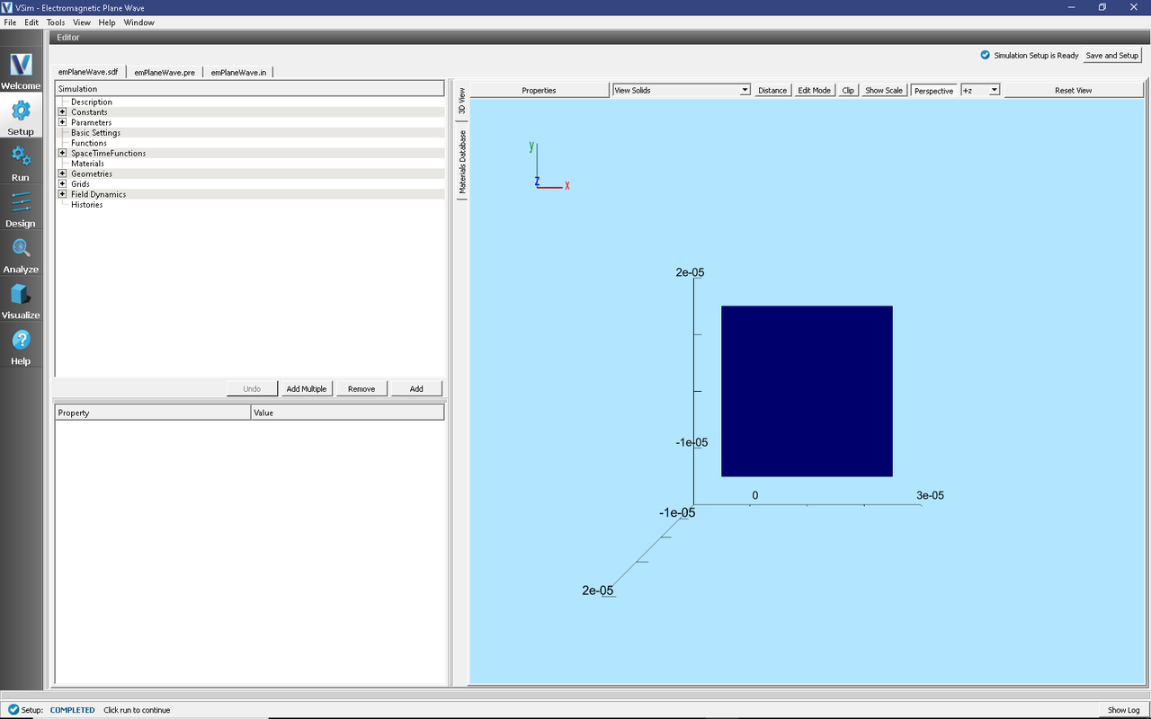
Fig. 157 Setup Window for the Electromagnetic Plane Wave example.
Simulation Properties
This example includes several constants for easy adjustment of simulation properties. Those include:
AMPLITUDE: The amplitude of the plane wave
WAVELENGTHS: The number of wavelengths inside the domain
There is a SpaceTimeFunction to define the plane wave that is launched with a Port Launcher boundary condition.
Running the Simulation
After performing the above actions, continue as follows:
Proceed to the Run Window by pressing the Run button in the left column of buttons.
To run the file, click on the Run button in the upper left corner of the Logs and Output Files pane. You will see the output of the run in the right pane. The run has completed when you see the output, “Engine completed successfully.” This is shown in Fig. 158.
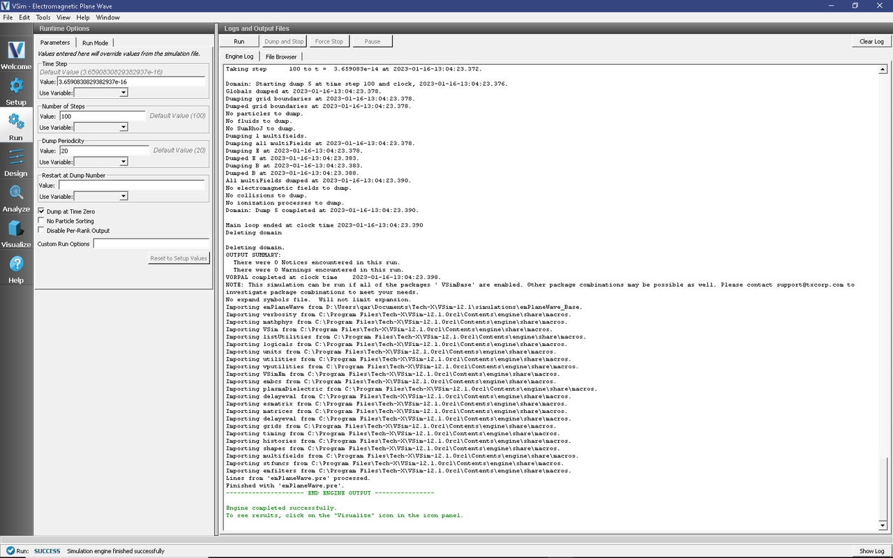
Fig. 158 The Run Window at the end of execution.
Visualizing the Results
After performing the above actions, continue as follows:
Proceed to the Visualize Window by pressing the Visualize button in the left column of buttons.
The electric and magnetic field components can be found in the scalar data variables of the data overview tab.
The Data Overview tab should be active. If it is not, click the Add a Data View dropdown below the toolbar and select Data Overview.
Here you can see Variables. Expand the Scalar Data.
Expand E
Select E_z
Initially, no field will be seen, as one is looking at Dump 0, the initial dump, when no fields are yet in the simulation. Move the slider at the bottom of the right pane to see the electric field at different times. The final time is shown in Fig. 159.
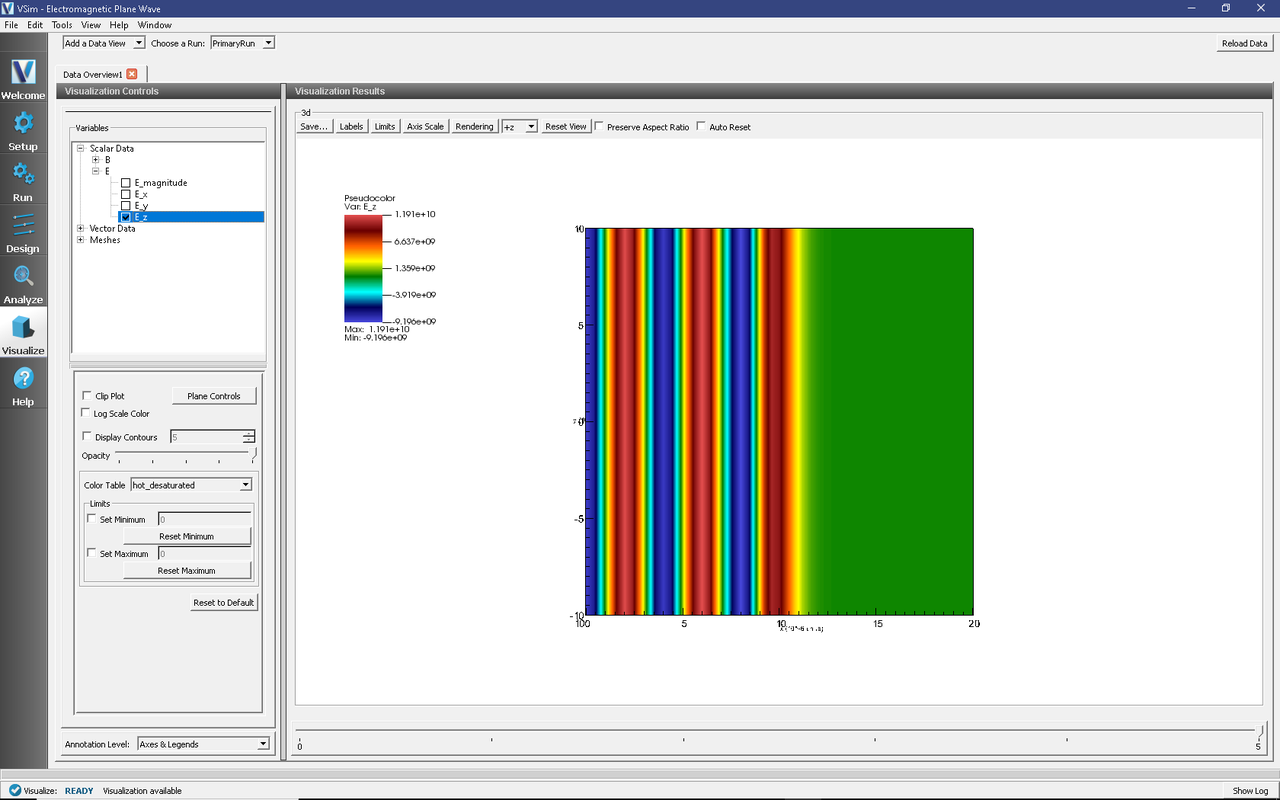
Fig. 159 Visualization of plane wave as a color contour plot.
Further Experiments
To see more wavelengths, change the value of the WAVELENGTHS variable. What happens to the waves when there are very few cells in a wavelength?
See the wave reflect off the right boundary by running for more time steps.
Try rotating the visualization by left-clicking and dragging with the mouse to see how the simulation is uniform across the z- dimension.