Kelvin-Helmholtz Instability (kelvinHelmholtz.sdf)
Keywords:
- fluid, periodic boundary
Problem description
This example demonstrates the Kelvin-Helmholtz instability that occurs in the presence of a velocity shear in a single, continuous fluid. The instability results in swirling eddies of fluid.
In this simulation, the density, flux, and energy density of a fluid are modeled via the Euler equations:
This problem demonstrates the Kelvin-Helmholtz instability for the case of a velocity difference across the interface between two different fluids that differ in density by a factor 2. A finite-width shear layer is used to ensure results converge at finite resolution. For the two-dimensional version of the problem setup considered here, we use a domain with periodic boundary conditions.
This simulation can be performed with a VSimBase license.
Opening the Simulation
The Kelvin Helmholtz example is accessed from within VSimComposer by the following actions:
Select the New → From Example… menu item in the File menu.
In the resulting Examples window expand the VSim for Basic Physics option.
Expand the Basic Examples option.
Select “Kelvin-Helmholtz” and press the Choose button.
In the resulting dialog, create a New Folder if desired, and press the Save button to create a copy of this example.
All of the properties and values that create the simulation are now available in the Setup Window as shown in Fig. 172.
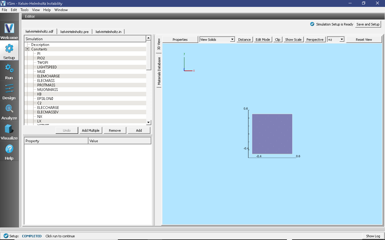
Fig. 172 Setup Window for the Kelvin-Helmholtz example.
Simulation Properties
Constants are set up to allow setting the number of cells (RESOLUTION), box length (BOX_LENGTH), CFL condition factor (CFL_FACTOR), number of timesteps (NSTEPS), pressure (P0), width of the initial perturbation (SWIDTH), initial density floor (D0), amplitude of the initial pressure perturbation (PAMP), and initial minimum flux (VFLOW).
Running the Simulation
After performing the above actions, continue as follows:
Proceed to the Run Window by pressing the Run button in the left column of buttons.
To run the file, click on the Run button in the upper left corner of the
Logs and Output Files* pane. You will see the output of the run in the right pane. The run has completed when you see the output, “Engine completed successfully.” A snapshot of the simulation run completion is shown in Fig. 173.
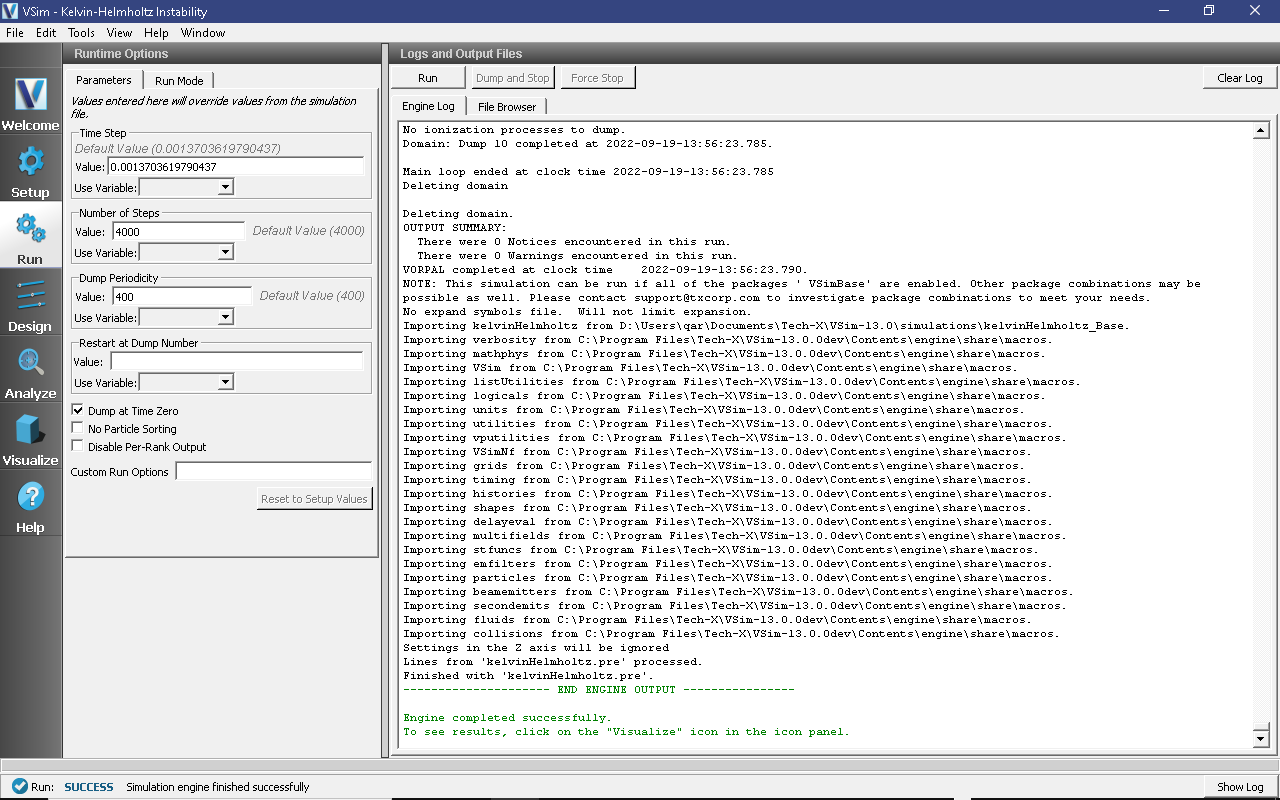
Fig. 173 The Run Window at the end of execution.
Visualizing the Results
The density shown in Fig. 174 shows the classic swirling structure that develops due to the Kelvin-Helmholtz instability.
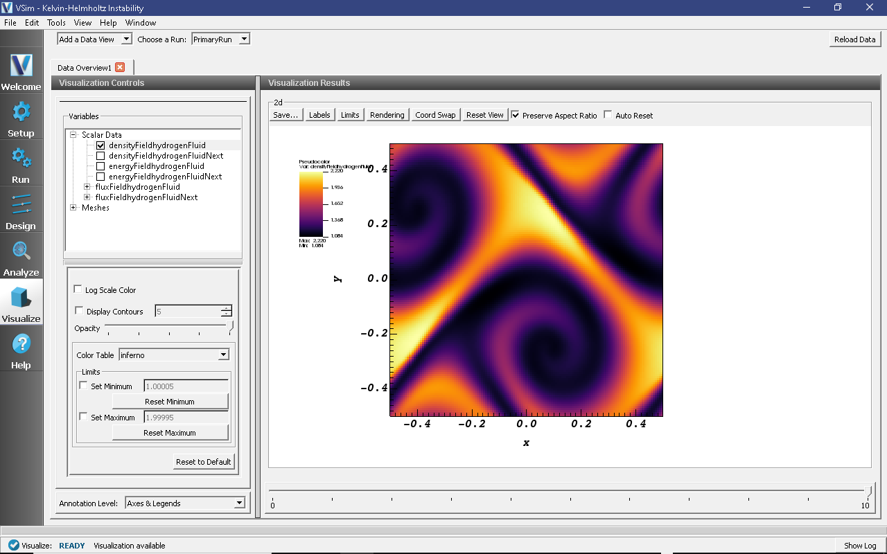
Fig. 174 The fluid density.