Oscillating Dipole Above Conducting Plane (emOscDipoleAboveConductor.sdf)
Keywords:
- emOscDipoleAboveConductor, radiation
Problem Description
This problem consists of an infinitesimally short dipole located at a variable height and orientation above a conducting plane. The simulation computes the electric and magnetic fields that can be visualized to show how the distance between, and orientation of the dipole relative to the conducting plane affects these fields.
This simulation can be performed with a VSimBase license.
Opening the Simulation
The Dipole Above Conducting Plane example is accessed from within VSimComposer by the following actions:
Select the New → From Example… menu item in the File menu.
In the resulting Examples window expand the VSim for Basic Physics option.
Expand the Basic Examples option.
Select Oscillating Dipole Above Conducting Plane and press the Choose button.
In the resulting dialog, create a New Folder if desired, and press the Save button to create a copy of this example.
All of the properties and values that create the simulation are now available
in the Setup Window as shown in Fig. 154.
You can expand the tree elements and navigate through the
various properties, making any changes you desire. The right pane shows a 3D
view of the geometry, if any, as well as the grid, if actively shown. To show
or hide the grid, expand the Grid element and select or deselect the box next
to Grid.
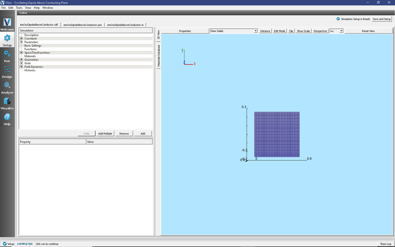
Fig. 154 Setup Window for the Dipole Above Conducting Plane example.
Simulation Properties
This example includes several constants for easy adjustment of simulation properties, Including:
AMPLITUDE: The amplitude of the dipole current
FREQUENCY: The operating frequency
There is also a SpaceTimeFunction to define the current driver of the dipole source
Other properties of the simulation include open boundaries on all sides except for the lower x boundary, which is a perfect electric conductor. A Dipole Current source is used to set the location of the dipole source.
Running the Simulation
After performing the above actions, continue as follows:
Proceed to the Run Window by pressing the Run button in the left column of buttons.
To run the file, click on the Run button in the upper left corner of the Logs and output Files pane. You will see the output of the run in the right pane. The run has completed when you see the output, “Engine completed successfully.” This is shown in Fig. 155.
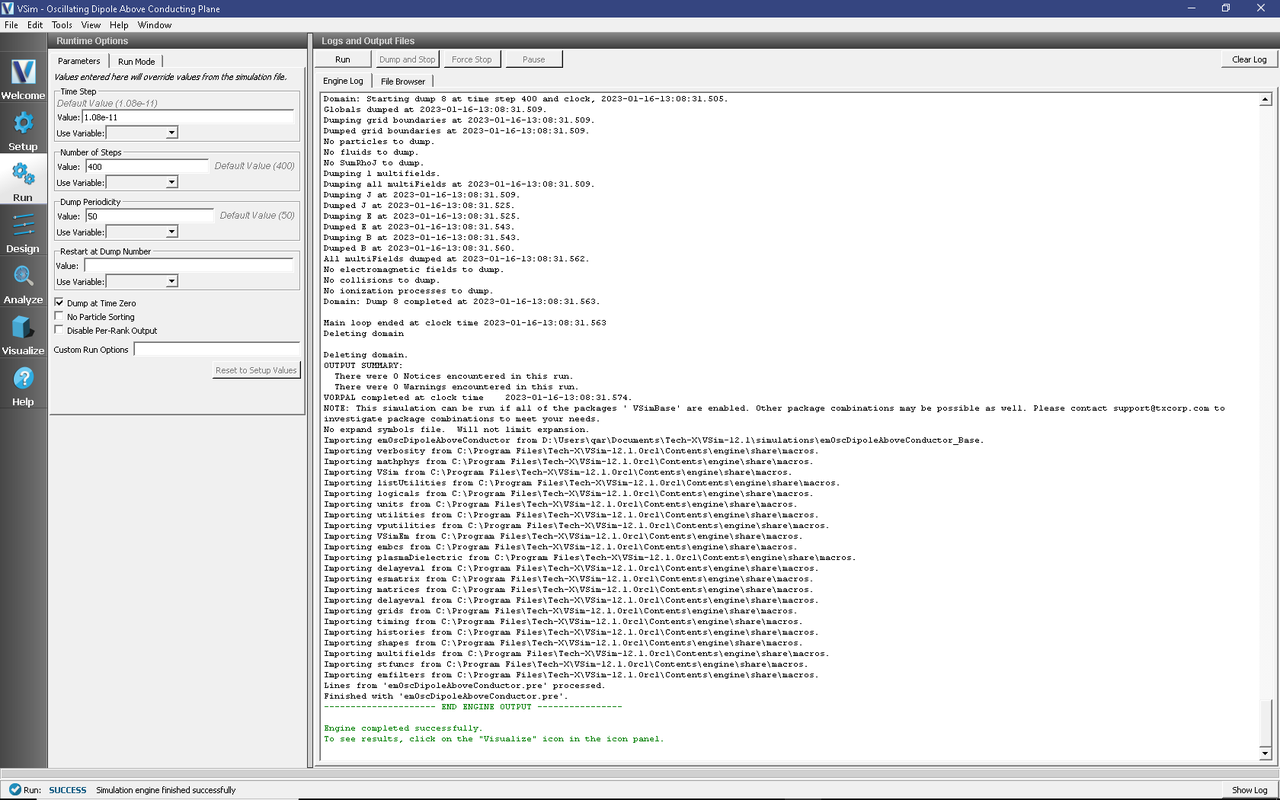
Fig. 155 The Run Window at the end of execution.
Visualizing the Results
After performing the above actions, continue as follows:
Proceed to the Visualize Window by pressing the Visualize button in the left column of buttons.
The electric and magnetic field components can be found in the scalar data variables of the data overview tab. To create the plot shown in Fig. 156 do the following:
Expand Scalar Data
Expand E
Select E_y
Select the box next to Display Contours and set the # of contours to 12
Select the box next to Clip All Plots
Drag the slider at the bottom of the Visualization Results pane to the right to show the 8th data dump
If desired, rotate the plot by clicking and dragging your mouse
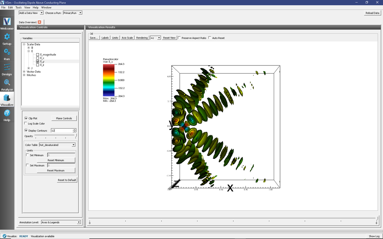
Fig. 156 The electric field
Further Experiments
In this example the “infinite” electric conductor is simulated by a physical conducting boundary at the bottom of the simulation. It would be possible to achieve the same results by having a second, equal infinitesimal dipole placed the same height “below” the conducting plane.
The number of “lobes” visible in the far field is dependent on Antenna Orientation and height. If vertically oriented there will be 2*Height/Wavelength +1 lobes.A horizontally oriented dipole will produce 2*Height/Wavelength lobes. This can be a bit difficult to visualize using just E-field data as it must be properly thresholded. The lobes will be easier to see in the example Advanced Dipole Above Conductor, a part of the VSimEM package.