Electrostatic Particle in Cell (esPtclInCell.sdf)
Keywords:
- electrostatics, particle in cell, sheath
Problem description
This Electrostatic Particle in Cell example computes the electrostatic potential and field in a box with conducting walls and particle absorbers and with an immobile, background neutralizing charge density. The electrons move to the wall by the potential, creating a sheath.
This simulation can be performed with a VSimBase license.
Opening the Simulation
The electrostatic particle in cell example is accessed from within VSimComposer by the following actions:
Select the New → From Example… menu item in the File menu.
In the resulting Examples window expand the VSim for Basic Physics option.
Expand the Basic Examples option.
Select Electrostatic Particle in Cell and press the Choose button.
In the resulting dialog, create a New Folder if desired, and press the Save button to create a copy of this example.
All of the properties and values that create the simulation are now available
in the Setup Window as shown in Fig. 166.
You can expand the tree elements and navigate through the
various properties, making any changes you desire. The right pane shows a 3D
view of the geometry, if any, as well as the grid, if actively shown. To show
or hide the grid, expand the Grid element and select or deselect the box next
to Grid.
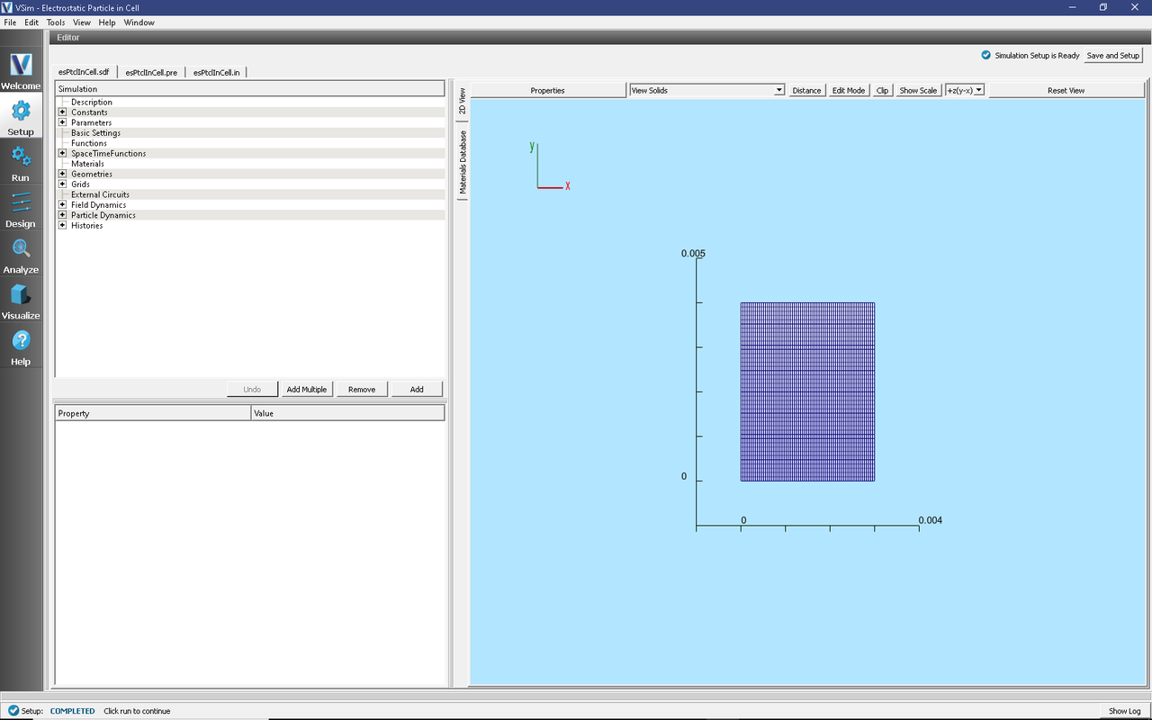
Fig. 166 Setup Window for the electrostatic particle in cell example.
Simulation Properties
This simulation includes several constants for easy adjustment of simulation properties including:
N_X, N_Y: The number of cells in each direction
W_X, W_Y: The length of the domain in each direction
PPC: The number of macroparticles per cell
The Parameters element contains several parameters useful for calculating basic plasma physics properties such as the plasma frequency and Debye length.
There is a SpaceTimeFunction used later in the setup to describe the thermal velocity of the electrons.
The simulation is periodic in y with Dirichlet boundary conditions in x set to zero.
Running the Simulation
After performing the above actions, continue as follows:
Proceed to the Run Window by pressing the Run button in the left column of buttons.
To run the file, click on the Run button in the upper left corner of the Logs and Output Files pane. You will see the output of the run in the right pane. The run has completed when you see the output, “Engine completed successfully.” A snapshot of the simulation run completion is shown in Fig. 167.
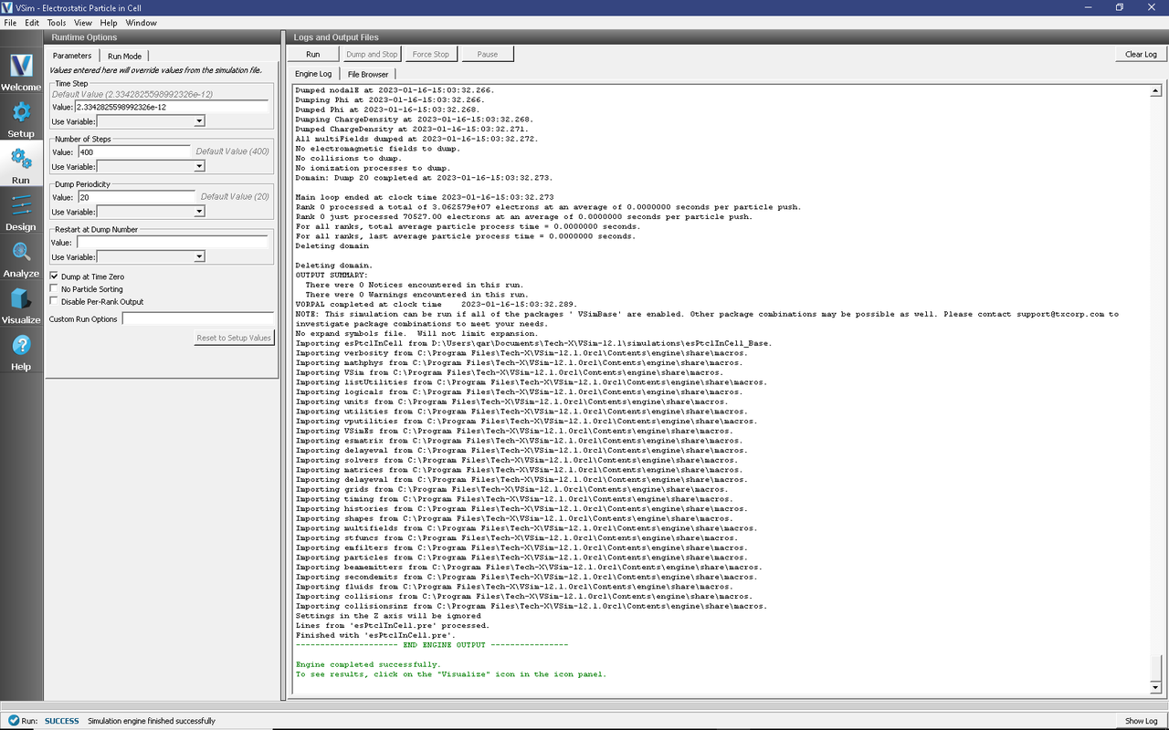
Fig. 167 The Run Window at the end of execution.
Visualizing the Results
After performing the above actions, continue as follows:
Proceed to the Visualize Window by pressing the Visualize button in the left column of buttons.
To view the electric potential as shown in Fig. 168, do the following:
Expand Scalar Data
Select Phi
Move the dump slider forward in time to see the evolution of the field.
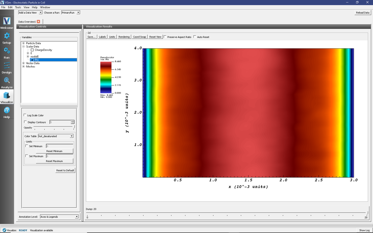
Fig. 168 The Visualize Window showing the electric potential, Phi, at dump 20.
Further Experiments
Change the plasma density and see whether the frequency in the histories changes.
Use the computePtclNumDensity analysis script in the Analyze Tab to calculate the electron density at each dump and view the sheath formation.