Parallel Plate Capacitor (parPlateCapacitor.sdf)
Keywords:
- electrostatics, parallel plate capacitor
Problem description
This Parallel Plate Capacitor simulation computes the electrostatic potential and field for a parallel plate capacitor. It can be run in any number of dimensions. It is periodic in the y and z directions when they are present.
This simulation can be performed with a VSimBase license.
Opening the Simulation
The Parallel Plate Capacitor example is accessed from within VSimComposer by the following actions:
Select the New → From Example… menu item in the File menu.
In the resulting Examples window expand the VSim for Basic Physics option.
Expand the Basic Examples option.
Select Parallel Plate Capacitor and press the Choose button.
In the resulting dialog, create a New Folder if desired, and press the Save button to create a copy of this example.
All of the properties and values that create the simulation are now available in the Setup Window as shown in Fig. 175. You can expand the tree elements and navigate through the various properties, making any changes you desire. The right pane shows a 3D view of the geometry, if any, as well as the grid, if actively shown. To show or hide the grid, expand the Grid element and select or deselect the box next to Grid
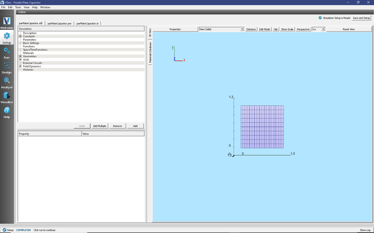
Fig. 175 Setup Window for the Parallel Plate Capacitor example.
Simulation Properties
The Simulation Elements Tree and Property Editor allow one to choose the distance between the plates, width of the plates, voltage of the positive plate and the length of a time step (which is irrelevant as this is an electrostatic simulation)
Running the Simulation
After performing the above actions, continue as follows:
Proceed to the Run Window by pressing the Run button in the left column of buttons.
To run the file, click on the Run button in the upper left corner of the Logs and output Files pane. You will see the output of the run in the right pane. The run has completed when you see the output, “Engine completed successfully.” This is shown in Fig. 176.
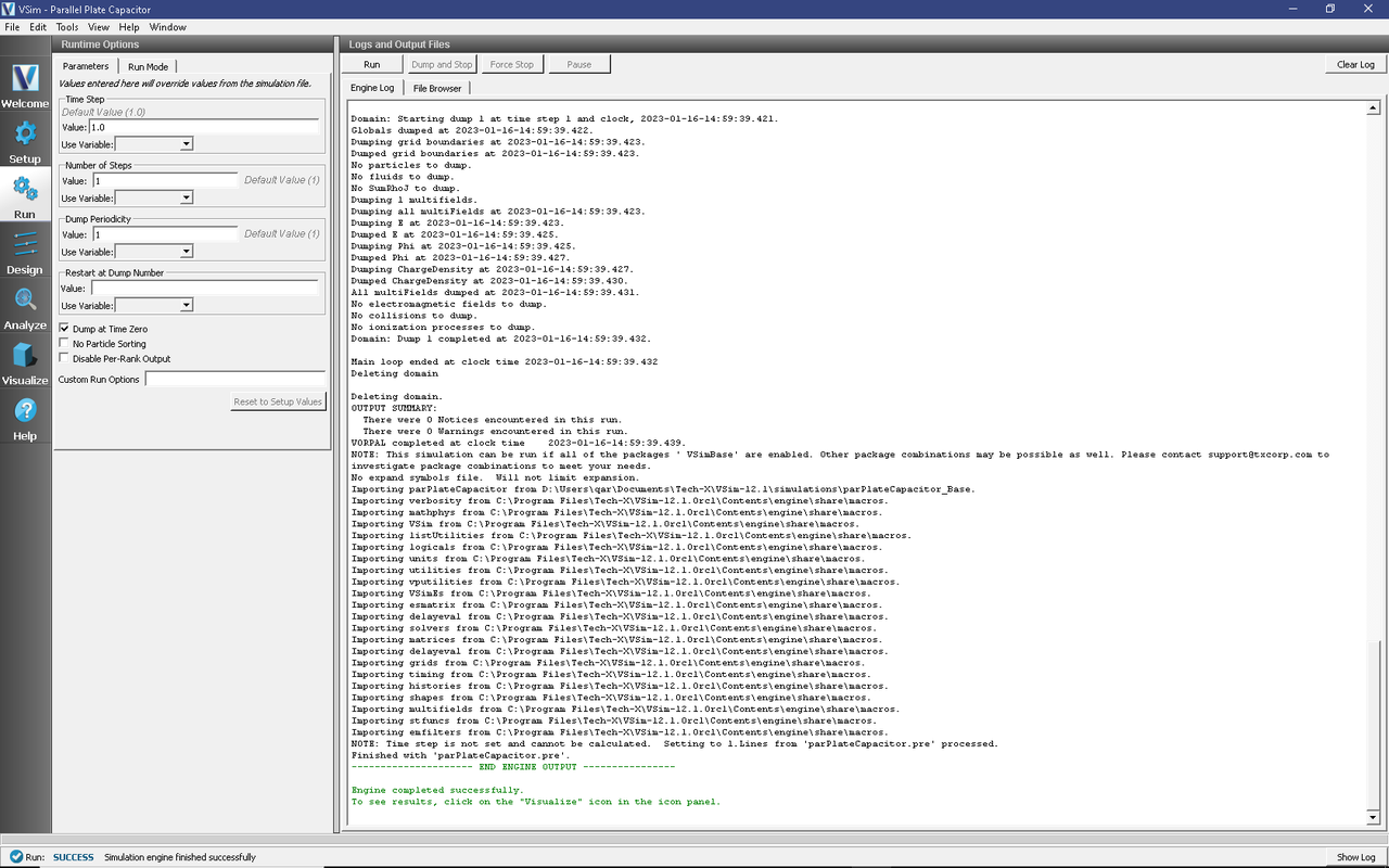
Fig. 176 The Run Window at the end of execution.
Visualizing the Results
After performing the above actions, continue as follows:
Proceed to the Visualize Window by pressing the Visualize button in the left column of buttons.
To create the image shown in Fig. 177, proceed as follows:
Expand Scalar Data and select the box next to Phi
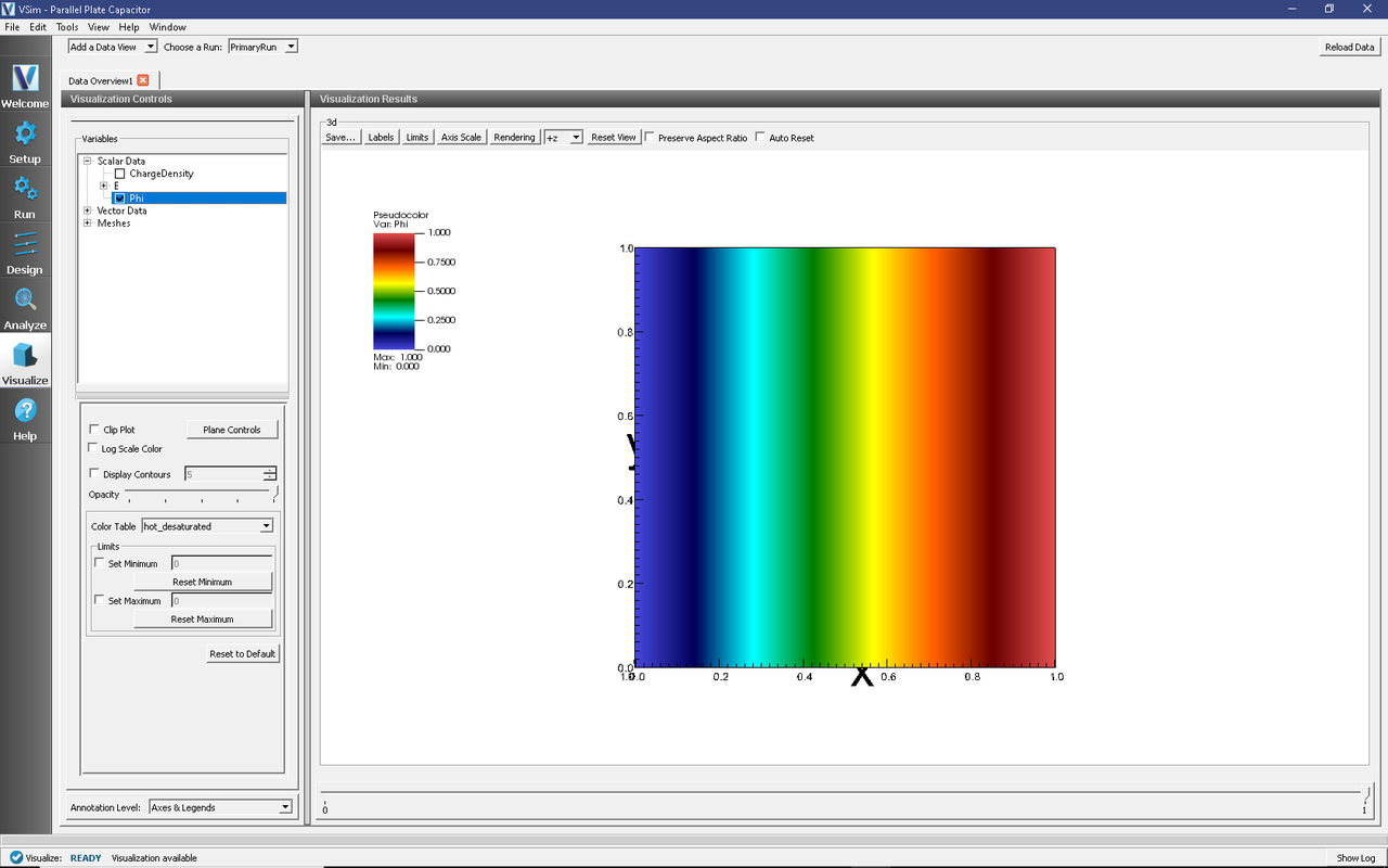
Fig. 177 Visualization of plane wave as a color contour plot.
Further Experiments
Change the gap between the plates by changing the length of the grid in the z direction and see how the electric field changes.
Change a width, e.g., LY and see whether it has an effect on the electric field.
Change the voltage on the right plate and see if it affects the electric field.
Set the periodic directions under BasicSettings to none, add boundary conditions on those directions and see how the field changes.