annnotateSpeciesDataOnPlane.py
This analyzer provides particle files corresponding to the data in the history.
-
-s<simname>,--simulationName=<simname> (string, required)
<simname> is the name of the simulation to be analyzed. The file extension should NOT be included in this text field.
-
-S<spname>,--speciesName=<spname> (string, required, default = electrons)
<spname> is the name of the species to analyze.
-
-H<histname>,--historyName=<histname> (string, required, default = speciesOnPlane)
<histname> is the name of the history to analyze.
-
-o<outspname>,--outputSpeciesName=<outspname> (string, optional, default = speciesOnPlane)
<outspname> is the name of the species file to write.
-
-w,--overwrite (flag)
Whether a dataset or group should be overwritten if it already exists.
Output
This analysis script produces particle vizschema hdf5 output corresponding to what passed through the plane.
If you are running this analyzer from the UI, and the output dataset file already exists, then it will be overwritten each time the analyzer is run, unless you uncheck the Overwrite Existing Files box near the bottom of the Analysis Results pane.
If you are running the analyzer from the command line, the dataset will not be overwritten
unless the -w, or --overwrite flag is specified on the command line.
The results of your analyzer may not be written into the output file if you have not specified the overwrite option to be True.
Example of Usage
Consider the electron gun simulation (text driven). You may add this block to measure the particles crossing a given plane.
<History speciesOnPlane>
  kind = speciesDataOnPlane
  initialPlanePos = $XEND-10.*DX$
  planeVelocity = 0.
  species = [electron]
</History>
This example may be run for 8000 steps and there may already be enough data recorded by this history to be worthwhile.
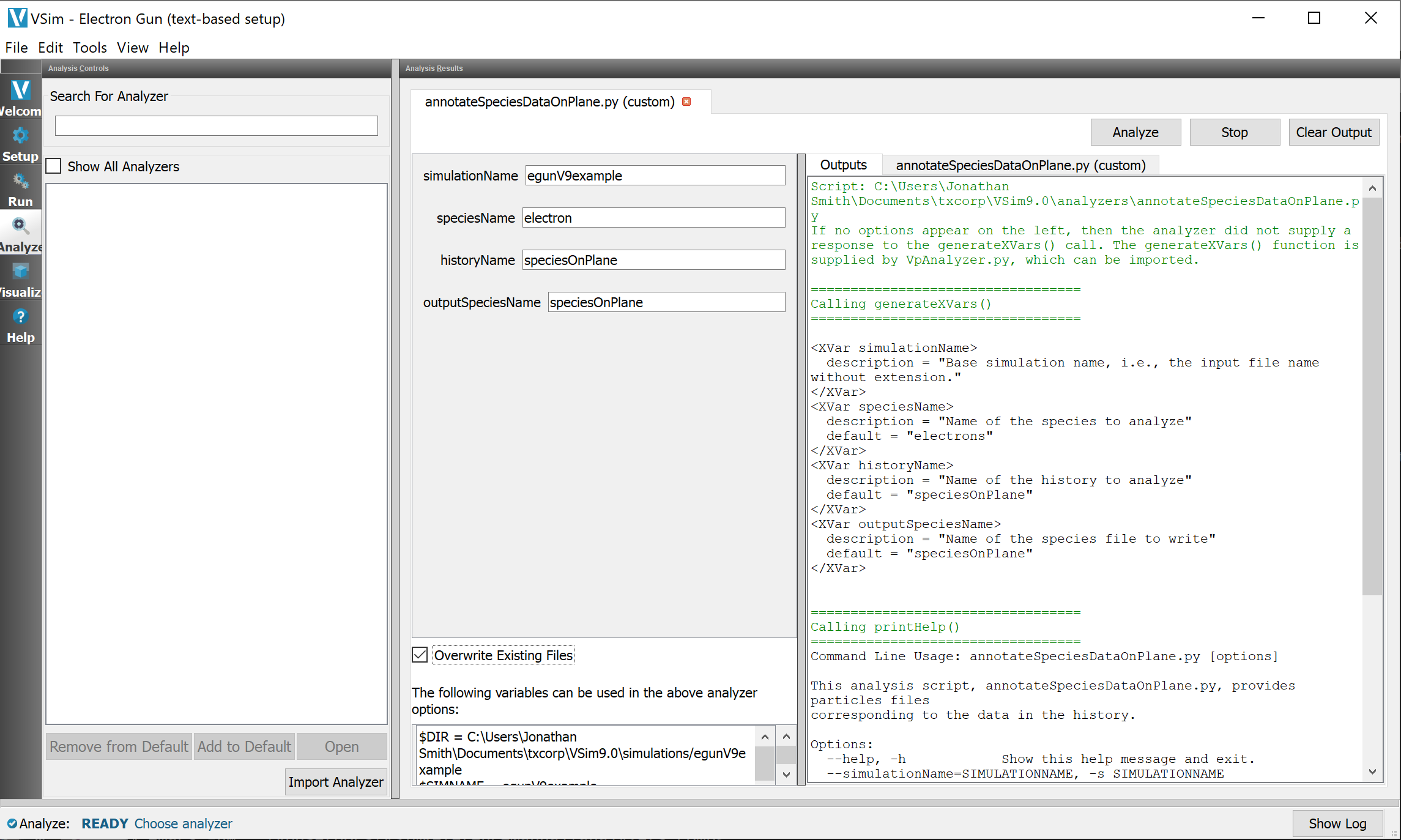
We can set the analyzer settings as shown in Fig. 606
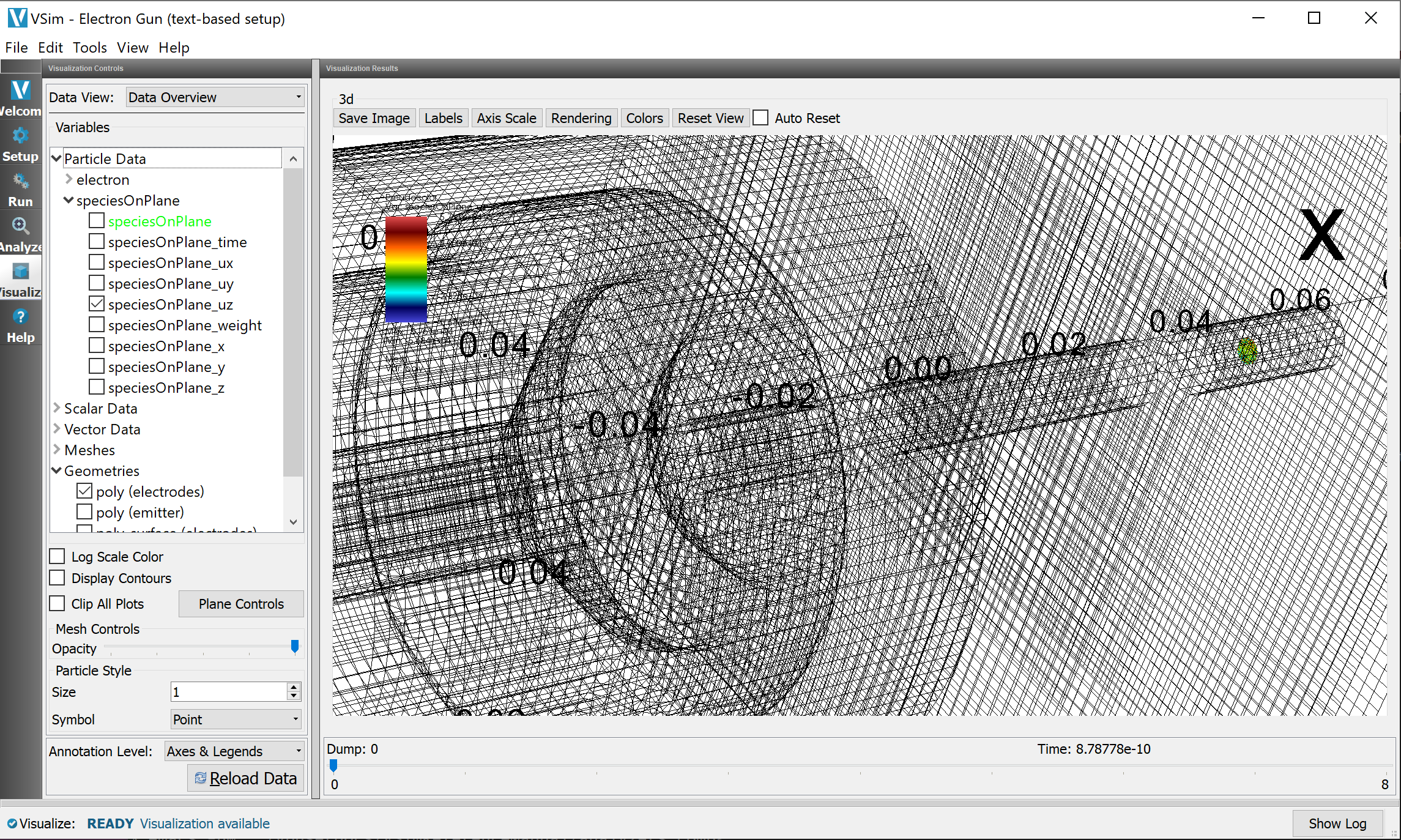
This will allow you to plot the particles collected by the history like any other species in the simulation as shown in Fig. 607
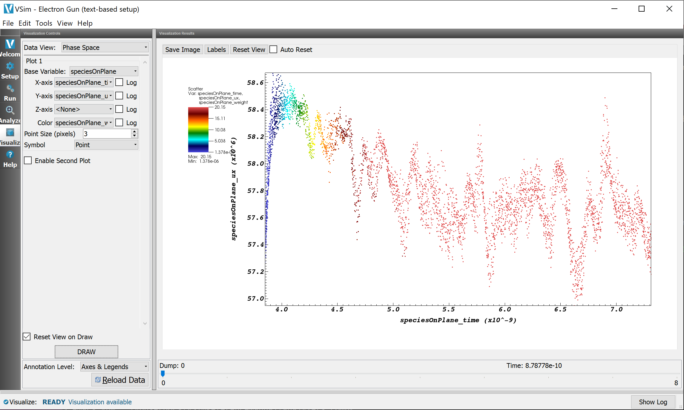
It also opens up other postprocessing opportunites, such as phase space plots and binning plots. In Fig. 608 we see the phase space, and the availability of the additional particle attribute representing time in the simulation. Longitudinal velocity is being plotted against time of arrival on the plane, coloured by the macroparticle weight - proportional to the number of physical particles per particle.


