Cylindrical Hall Thruster (cylHallThruster.sdf)

Problem description

Electric Hall thrusters are used for in-space propulsion and satellite station-keeping needs. The discharge plasma inside the Hall thruster channel is produced by the ionization of electrons with a neutral propellant gas such as xenon. The electrons are emitted from the neutralizer cathode placed at the exit of the Hall thruster (cathode end). The neutral gas is fed into the channel from the anode end of the Hall thruster channel. The electrons are confined inside the Hall thruster channel by the radial magnetic field applied through the solenoidal magnetic fields. Plasma xenon ions are accelerated out of the channel at high velocity, which produces the thrust necessary for space propulsion. Recently these thrusters are being designed to support long life time, high-power and high-thrust operations. The channel wall erosion occurring inside of the Hall thruster is one of the main limitations to these design needs. It becomes important to understand the plasma discharge processes occurring inside the Hall thruster channel and predict the lifetime of the Hall thruster based on the calculations of sputtered material from the Hall thruster channel.

This example demonstrates elements of the full cylindrical Hall thruster text-based example. Please refer to that documentation for a detailed description of the simulation geometry, and physical properties of the full model. This visual-setup model employs the same physical geometry (2D, cylindrical coordinates) as the text-based setup model. As with the text-based setup example, there is an electron source and a background xenon gas that is ionized by kinetic electrons to produce kinetic xenon ion particles. Particle sinks, and the physical extent of the background gas are the same as in the text-based example.

The primary difference is that there are no dielectric materials in this example, and so the electromagnetic fields are different. This leads to a different pattern for electrons exiting the simulation than in the text-based example. Also, there is no neutral particle sputtering of wall material included in this example. This example does demonstrate ionization of neutral gas in cylindrical geometry.

This simulation can be performed with a VSimPD license.

Opening the Simulation

The Cylindrical Hall Thruster example is accessed from within VSimComposer by the following actions:

• Select the New → From Example… menu item in the File menu.
• In the resulting Examples window expand the VSim for Plasma Discharges option.
• Expand the Spacecraft option.
• Select Cylindrical Hall Thruster and press the Choose button.
• In the resulting dialog, create a New Folder if desired, and press the Save button to create a copy of this example.

All of the properties and values that create the simulation are now available in the Setup Window as shown in Fig. 556. You can expand the tree elements and navigate through the various properties, making any changes you desire. The right pane shows a 3D view of the geometry, if any, as well as the grid, if actively shown. To show or hide the grid, expand the Grid element and select or deselect the box next to Grid.

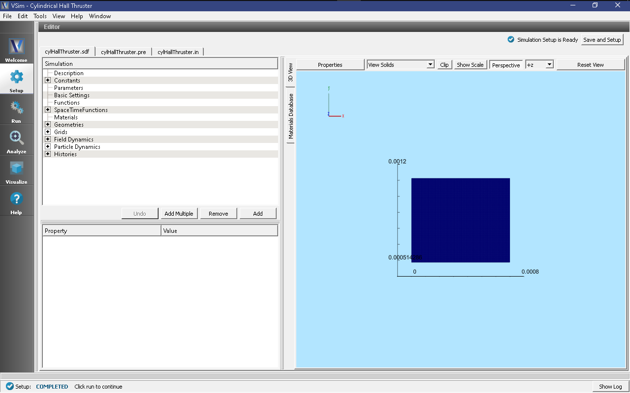
Fig. 556 Setup Window for the Cylindrical Hall Thruster Channel example.

Simulation Properties

This example contains many user defined Constants which help simplify the setup and make it easy to modify. These include constants such as:

• B0: The amplitude of the background magnetic field
• anodeV: the anode voltage
• innerRad and outerRad: inner and outer cylinder radius
• xeMaxDensity: the maximum density of the background Xe gas

There are also several SpaceTimeFunctions that are used to define spatially and/or temporally varying inputs to other properties. These include:

• By: the magnetic field profile
• initialGasDensity: the profile for the background gas density

The self-consistent electric field is solved from Poisson’s equation by the electrostatic solver in a cylindrical coordinate system. The simulation is performed in axisymmetric 2-D fashion. The plasma is represented by macro-particles which are moved using the Boris pusher in cylindrical coordinate system. Various types of elastic and inelastic collisions of the particles are also taken into account.

Running the simulation

After performing the above actions, continue as follows:

• Proceed to the Run Window by pressing the Run button in the left column of buttons.
• To run the file, click on the Run button in the upper left corner of the Logs and Output Files pane. You will see the output of the run in this pane. The run has completed when you see the output, “Engine completed successfully.” A snapshot of the simulation run completion is shown in Fig. 557.

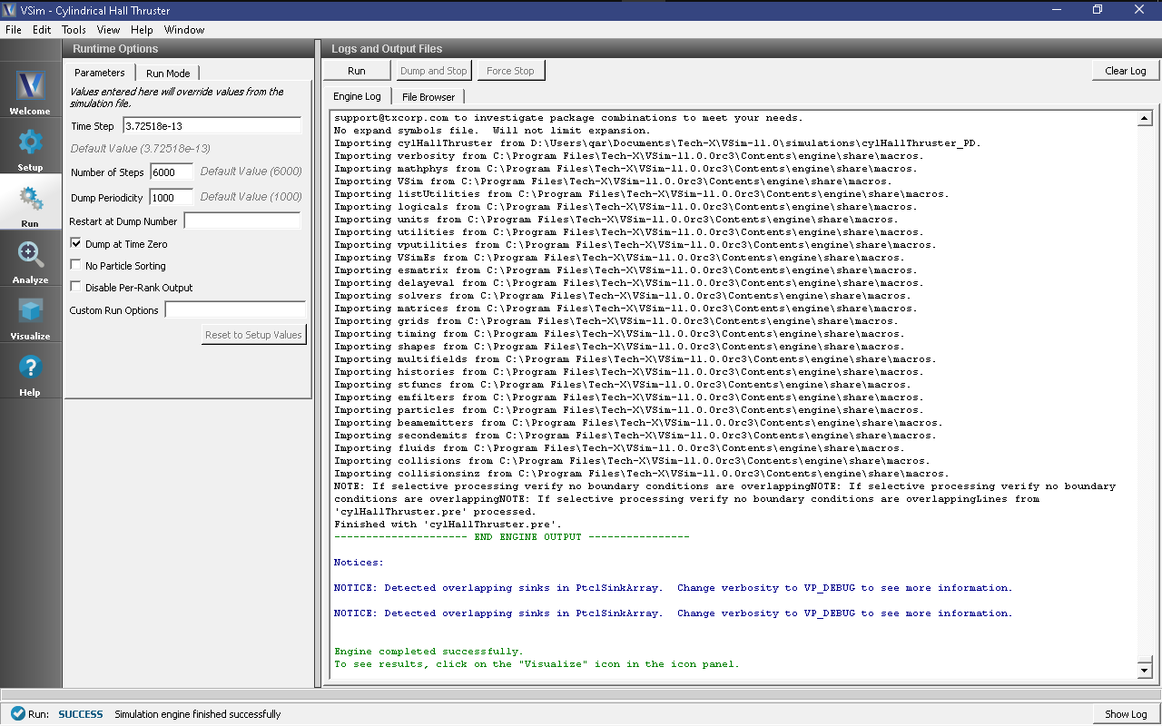
Fig. 557 The Run Window at the end of execution.

On an 8 core I7-6000 CPU, it takes about 40 minutes to run for 6,000 time steps. To reach steady state, about 100,000 time steps are required.

Analyzing the Results

If it is desired to calculate the density of the electrons or ions the analysis script computePtclNumDensity.py must be used.

• First click on the Analyze Tab.
• From the Available Anaylzers list, choose computePtclNumDensity.py. Then click Open.
• This script accepts the simulationName (Name of the input file) and speciesName to be calculated (species of particles).
• To calculate the density of the electrons, set the simulationName to “cylHallThruster” and the speciesName to “electrons”.
• Click on the Analyze button at the top right of the Analysis Results pane.
• A snapshot of the simulation run completion is shown in Fig. 558.

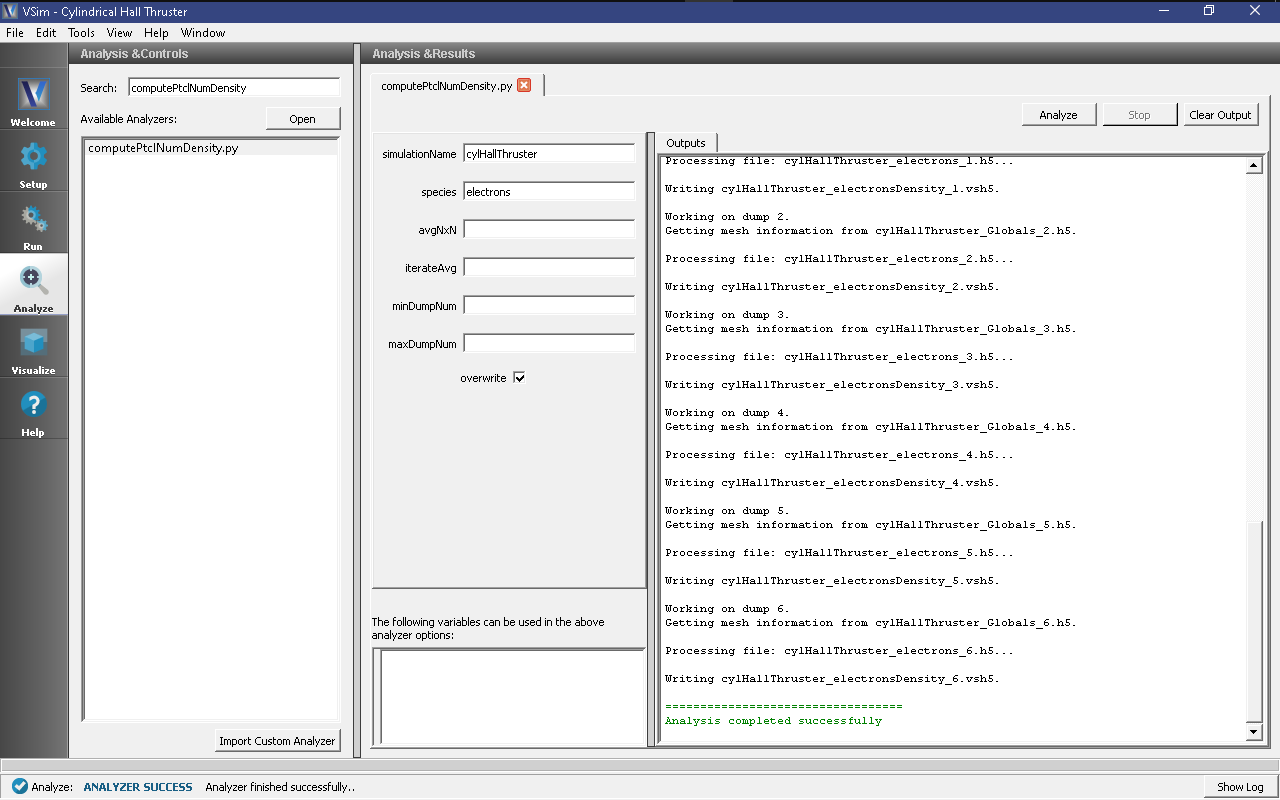
Fig. 558 The Analyze Window at the end of execution.

The resulting data will be visualizable as electronsDensity under the Scalar Data menu in the Visualize Tab. The density of other particles such as heavyIons, or Xeplus can also be calculated if those species names are used in place of electrons.

Visualizing the Results

To visualize the results, continue as follows:

• Proceed to the Visualize Window by pressing the Visualize button in the left column of buttons.

There are many different fields, particles, and histories that can be visualized in this example. The horizontal axis represents Z direction and the vertical axis represents R direction.

To view the electric potential, switch to the Data View to Data Overview in the Controls pane. Expand Scalar Data and choose Phi. Move the Dump slider to the right most position. Fig. 559 shows the visualization seen for the electric potential of the cylindrical Hall thruster channel and in the exit region.

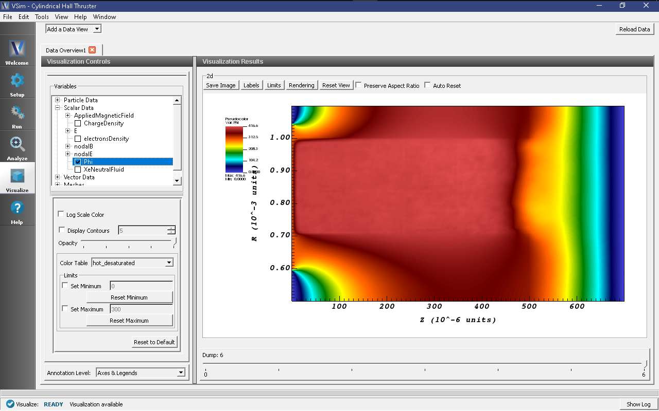
Fig. 559 Visualization of Cylindrical Hall thruster channel electric potential results.

In the Hall thruster channel plasma, the electrons injected from the right end (i.e., exit of the channel) are accelerated towards the anode biased wall at the left end. To plot the particles, expand Particle Data and select “electrons” and “XePlus” check boxes The figure below, Fig. 560, shows the distribution of positively charged xenon ions (red dots) and electrons (blue dots).

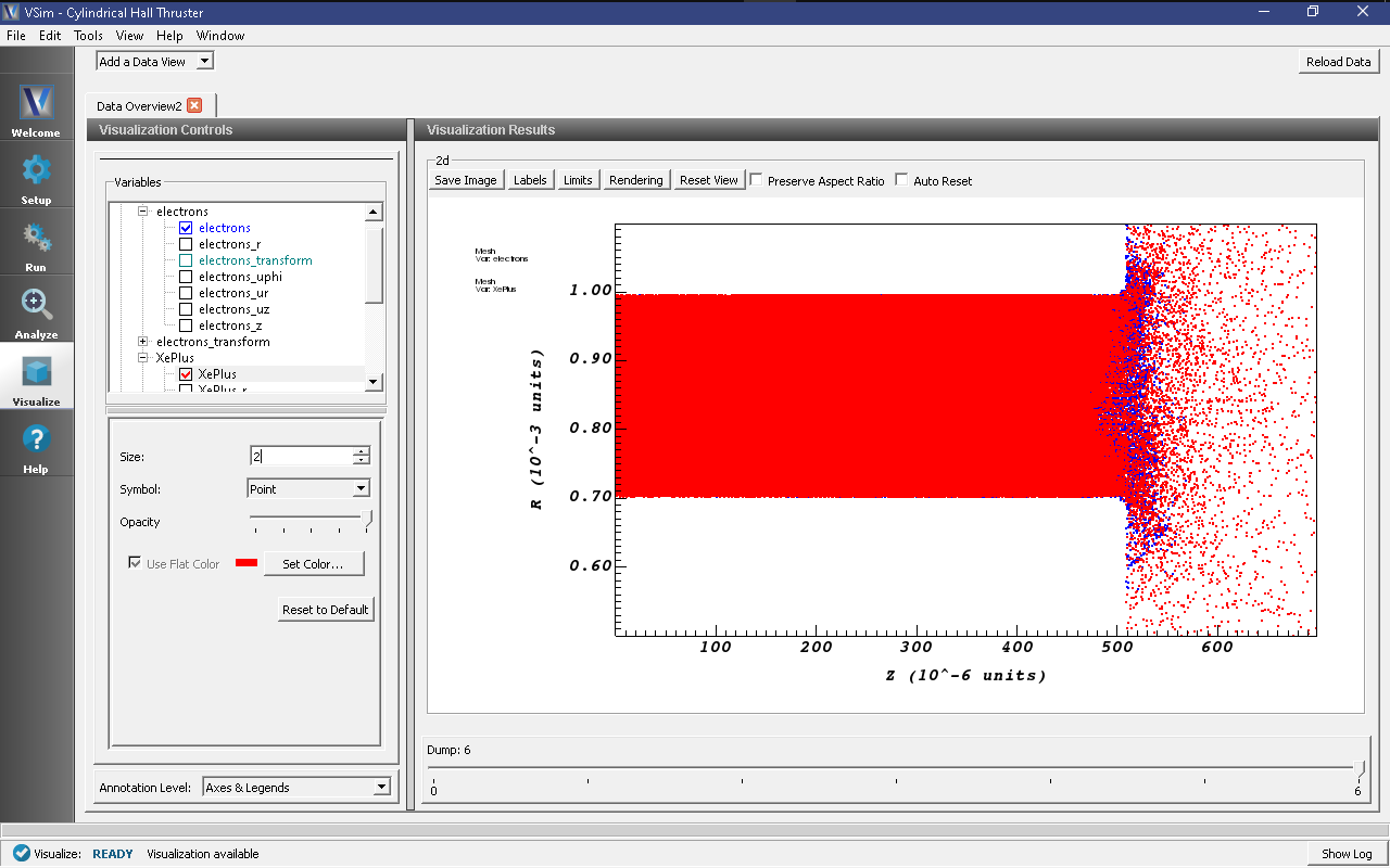
Fig. 560 Visualization of Cylindrical Hall thruster channel particle phase-space distribution results.

The static radial magnetic field distribution considered for the SPT-100 Hall thruster channel set up is shown in Fig. 561. To reproduce this plot, expand Scalar Data then nodalB and select nodalB_r. The magnetic field is strong near the inner cylinder and has a Gaussian bell-shaped field distribution both inside and at the exit of the channel.

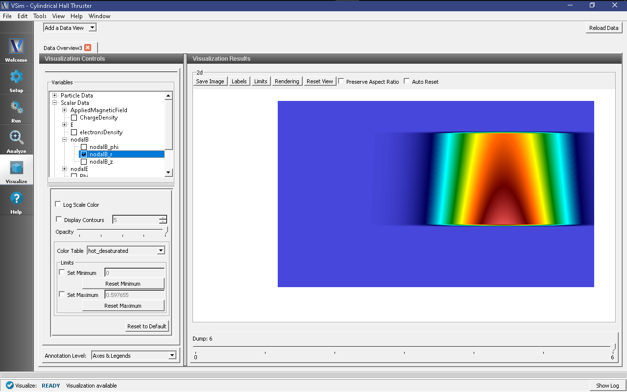
Fig. 561 Visualization of radial magnetic field in the Cylindrical Hall thruster channel.

The background xenon neutral gas density distribution (plottable as XeNeutralFluid under Scalar Data) used in the simulation set up is shown in Fig. 562. The maximum neutral gas density is taken at the left end of the channel near the anode wall. A linearly varying neutral gas density is assumed.

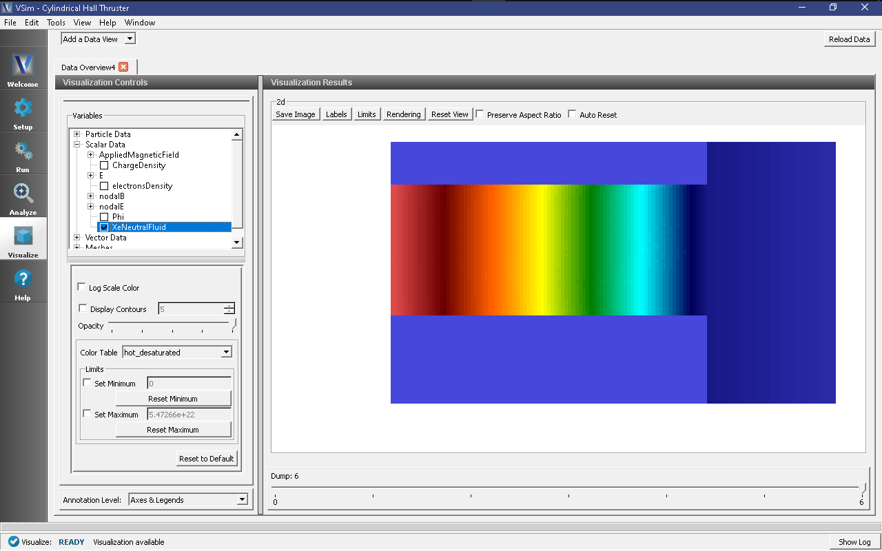
Fig. 562 Visualization of xenon neutral gas density in the Cylindrical Hall thruster channel.

Further Experiments

This example can be modified to test different design parameters such as varying anode voltages, varying background neutral gas densities and varying electron emission currents. This will allow users to study high-to-low power and high-to-low throttle levels.

Also the background gas type can be changed to investigate other neutral gas kinds in this simulation set up.