Townsend Discharge (townsend.sdf)

Problem Description

In a Townsend avalanche, electrons are accelerated by an electric field and ionize a background gas of neutral atoms or molecules. Each ionization event creates an additional electron that will also be accelerated and eventually produce more ionization events of its own. This process of repeated doubling results in an exponential increase in the number of electrons. The Townsend avalanche occurs when the electron and ion densities are too low to behave collectively and form a plasma.

This type of discharge is named after John Townsend who first proposed the ionization model to explain the phenomena. In his experiments, Townsend measured the current across a gas-filled chamber with a of pair of parallel plates on the two ends. Townsend illuminated the cathode plate with X-rays which produced electrons via the photo-electric effect. Townsend noticed that the current between the plates depended on the strength of the electric field between the plats and the pressure of the gas.

His observations lead to the conclusion that electrons were ionizing the gas and causing an exponential increase in the measured current. The current measured across the discharge chamber is described by the following formula:

where \(I_0\) is the photo-current produced by the X-rays, \(I(x)\) is the current through the chamber as a function of the plate separation, \(x\). The parameter \(x_0\) is a characteristic distance that a collection of electrons has to travel away from the cathode before an equilibrium is reached. The parameters \(\alpha\) and \(\gamma\) are the first and second Townsend coefficients, respectively. The first Townsend coefficient, \(\alpha\) is a measure of how many ionization events a single electron will produce per unit length, and \(\gamma\) is a parameter accounting for electron generation from secondary processes, like ion impact at the cathode.

In this example simulation, we will loosely follow the experimental setup of L.M. Chanin and G.D. Rork who measured the first Townsend coefficient for Helium [CR64a], Neon, and Hydrogen [CR64b] in the 1960s. For low voltage discharges, the factor \(\gamma\) is negligible and the equation above reduces to

In reality, \(\alpha\) is a complicated function of pressure, accelerating field, and the species of background gas molecule/atom. Chapter 14 section 3 of Principles of Plasma Discharges and Materials Processing, [LL05] presents an analytical model for \(\alpha\) as a function of pressure and electric field and provides the fitting constants for different gases. This simulation will estimate a value for \(\alpha\) for a Helium gas keeping the electric field and pressure constant at \(E = 2.12e5\) V/m and \(p = 21.2\) torr. At this pressure and electric field, the accepted value for \(\alpha\) is 1.3 [CR64a], [LL05].

This simulation can be run with a VSimPD license.

Opening the Simulation

The Townsend Avalanche example is accessed from within VSimComposer by the following actions:

• Select the New → From Example… menu item in the File menu.
• In the resulting Examples window expand the VSim for Plasma Discharges option.
• Expand the Processes option.
• Select Townsend Avalanche and press the Choose button.
• In the resulting dialog box, create a New Folder if desired, then press the Save button to create a copy of this example.

The resulting Setup Window is shown Fig. 537.

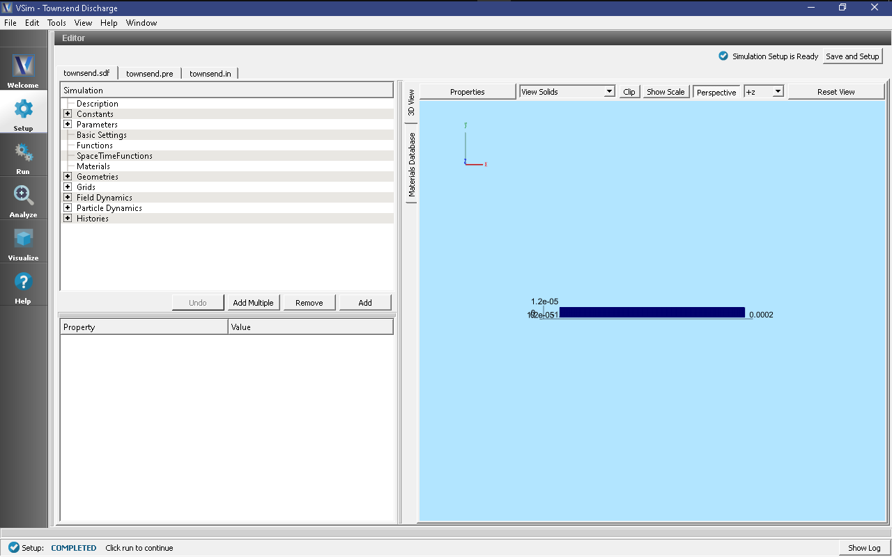
Fig. 537 Setup Window for the Townsend Avalanche example.

Simulation Properties

In order to calculate a value for the Townsend coefficient, this simulation will need to be run multiple times at different plate separations while keeping the electric field and pressure constant. The data points from these multiple runs will be used in a least squares fit to an exponential function of the form

where \(\alpha\) and \(\beta\) are the constants being fitted, with \(\alpha\) being the Townsend coefficient of interest. Details on how to fit the data yourself is covered in the section Computing the Townsend Coefficient below.

The simulation input file is set up to allow for rapid iteration on the multiple plate separations. The voltageDifference actually controls the separation of the two plates in such a way that keeps the electric field constant, and also is used to calculate an estimate for the maximum electron speed which goes into determining the time step.

In Basic Settings the field solver is set to prescribed fields. This means we manually set the electric field as a function of space (and have an option on add time dependence). In the Field Dynamics element, under Fields is where we actually set the value for the constant electric field present between the two plates at either end of the discharge tube. In the externalElectricField element we set component0, the x-component of the electric field to a value calculated from the parameters in [CR64a].

The Particle Dynamics element is where we set up the which particle species the simulation will contain, how particles of each species get added and removed from the simulation, and in what processes/interactions they participate.

This simulation contains an electron species, a positive helium ion species, and a background gas of helium neutral gas. The settableFluxSlabElectronEmitterCW0 is set up to emit a total of 100,000 physical electrons. Both the electron and helium ion species have been set up such that each macro particle corresponds to a single physical particle.

The electric field points from upper x (right side of screen) to lower x (left side of screen). The electrons are emitted into the simulation from the lower x and are accelerated to the right. There are seven interactions in which an electron can be involved as it crosses the simulation grid. These processes are set in the Reactions element, which has been enabled by choosing include particles and reactions in Basic Settings.

The processes included in this simulation are electron/neutral helium elastic scattering, five different electron/neutral helium excitation processes in which electrons lose some energy to putting a neutral helium atom into an excited state, and an electron/neutral helium ionization process which is the crucial bit of physics for this simulation. We found that the it was important to use the reaction type Inelastic Electron Scattering with scatter type set to VahediSurendra for getting an accurate value for the Townsend coefficient.

To add collision processes to VSim, cross-sections data must be supplied by the user. To get the most accurate results from this validation study, we used cross sections from the LxCat database. According to the terms of the database, we are not permitted to distribute data obtained from the database, so the data included as part of this example is less accurate. The following section provides a set of instructions for obtaining the more accurate cross-section data for yourself.

Downloading Cross-Sections from LxCat Database

In our validation study, the cross-sections used in the elastic, excitation, and ionization interactions between the electrons and the background neutral Helium gas were taken from the LxCat Database.

The terms of use of the LxCat database do not allow Tech-X to distribute the cross sections we used in our study which calculated a Townsend coefficient within 10% of accepted value of 1.31. Instead, less accurate estimates of the cross-sections are provided so that the simulation can will run.

To obtain a more accurate set of cross-sections from the LxCat Database, follow these instructions:

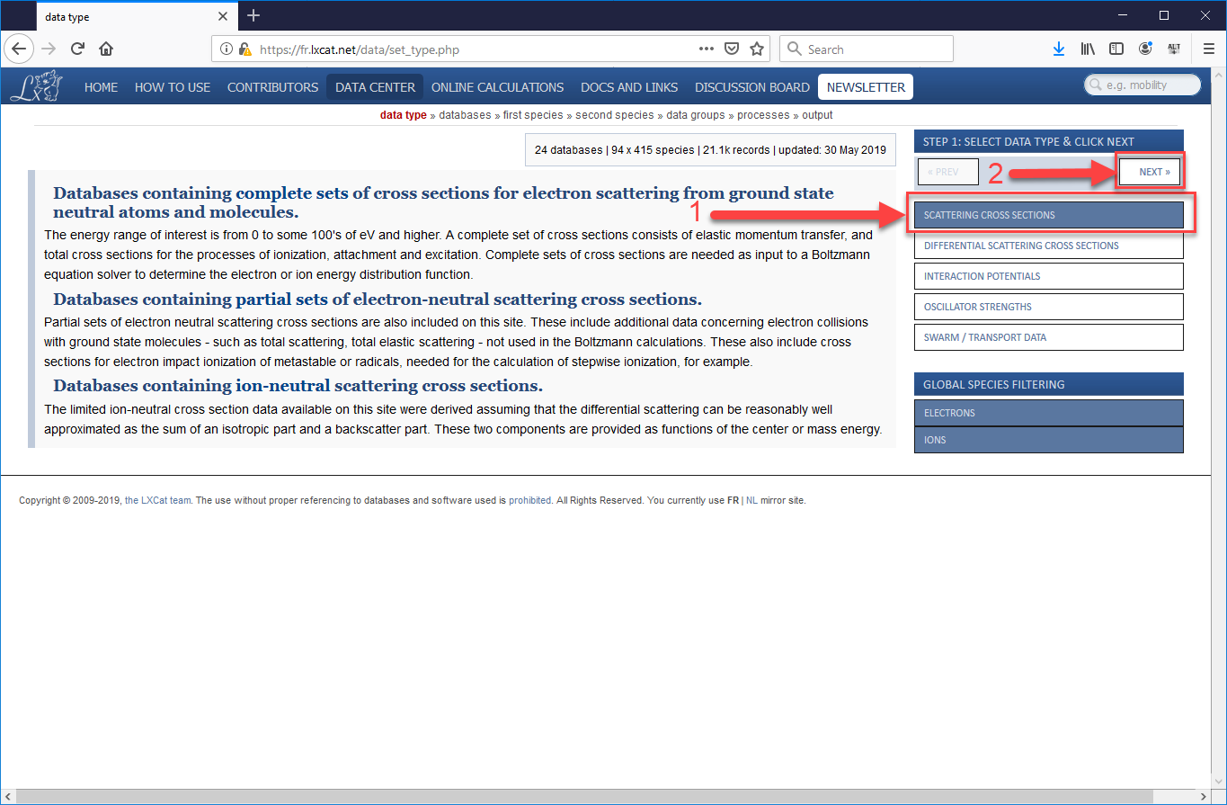
1. Open a Browser and follow this (https://fr.lxcat.net/data/set_type.php) link to the database.
2. From the menu bar on the left, select “Scattering Cross Sections” and press “Next.”

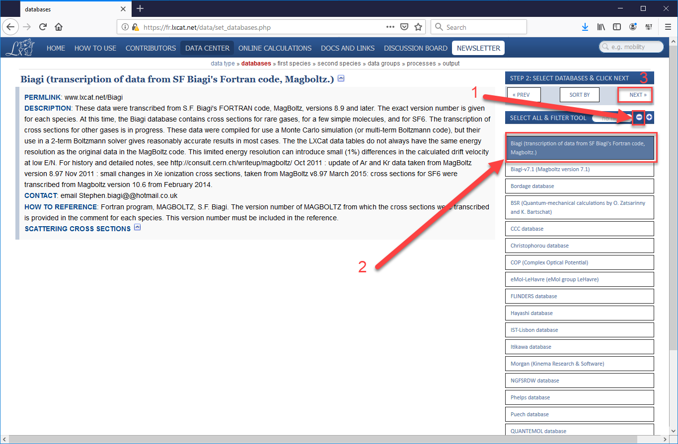
3. On the next page, first press the “minus” button to de-select all options, then select the “Biagi (transcription of data from SF Biagi’s Fortan code, Magboltz.)” Alternatively, you could choose another sub-database from which to obtain cross-sections, the data from all the sources agree fairly well, but we are taking you to the specific set we used in our validation study. After the sub-database is selected, press “Next”.

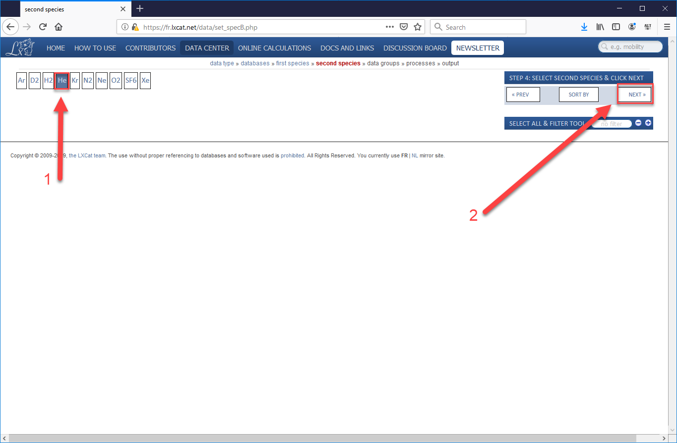
4. Since we are using the Biagi data, which are all processes which involve electrons, we skip over the choice of first species (since it will be an electron) and go straight to choosing the second species. Choose “He” (or your species of choice), then “Next”.

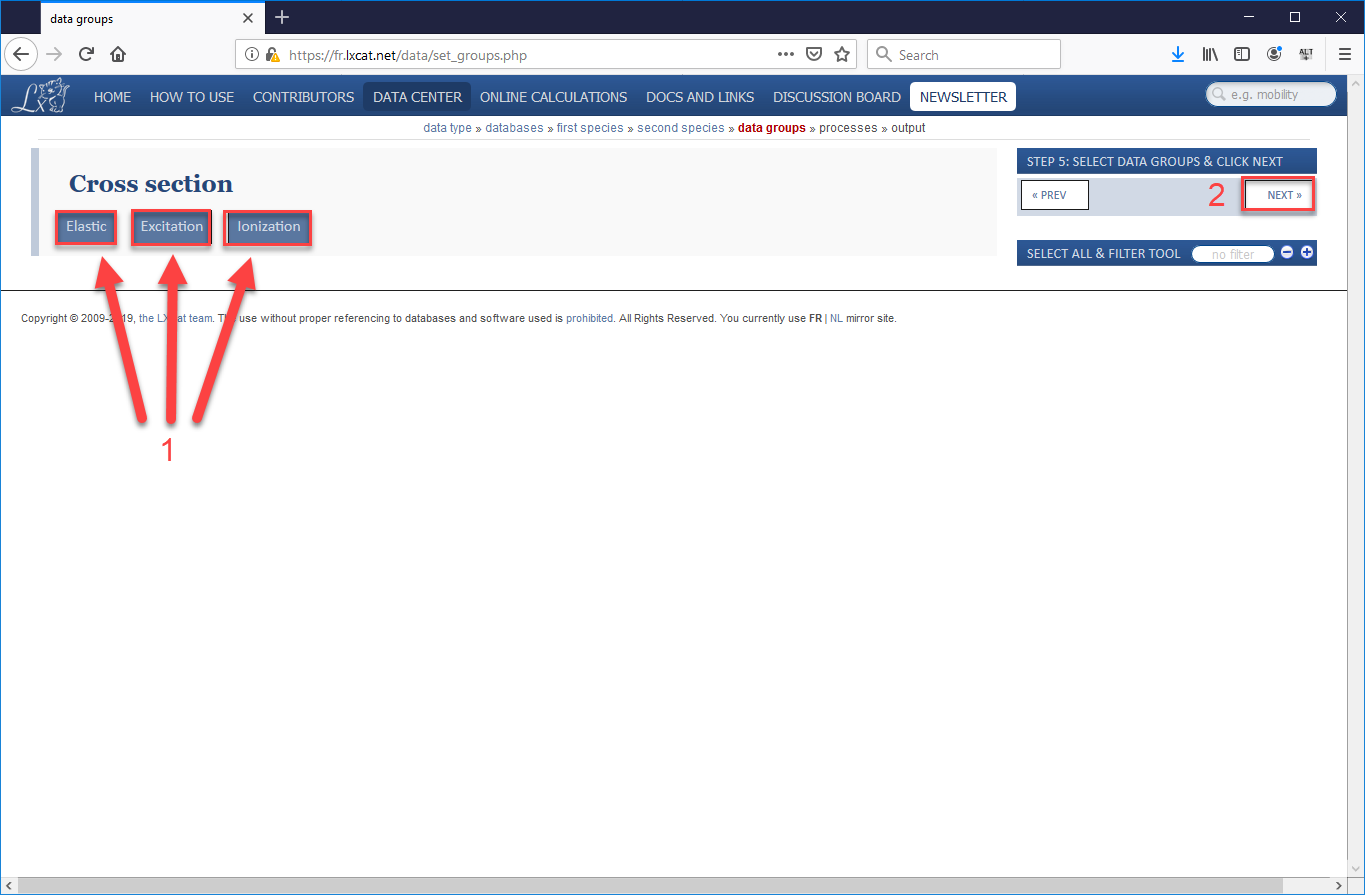
5. We will be using Elastic Scattering, Excitation, and Ionization processes for this simulation, so select all three options (“Elastic”, “Excitation”, and “Ionization”) the press “Next”.

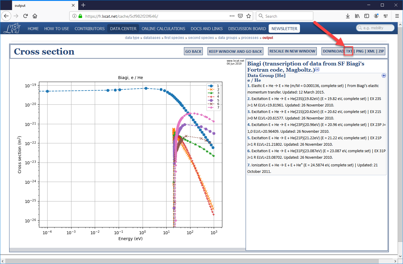
6. One the next page that opens will be a long list of electron-helium processes, the majority of which will be excitation processes which involve an electron passing energy to a neutral helium atom, sending it into an excited state, which will eventually cause the helium atom to emit a photon (which will not be tracked in VSim) when the atom returns to its ground state. In our validation study, we used the cross-sections for the elastic scattering process, five of the most common excitation processes, and the ionization process. Be sure to check the boxes for all 7 processes, scrolling down to the very bottom to find ionization (as shown in images Fig. 542 and Fig. 543). Then scroll back up and press “Next”.

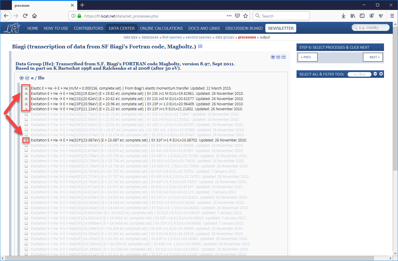
Fig. 542 LxCat Step 6a

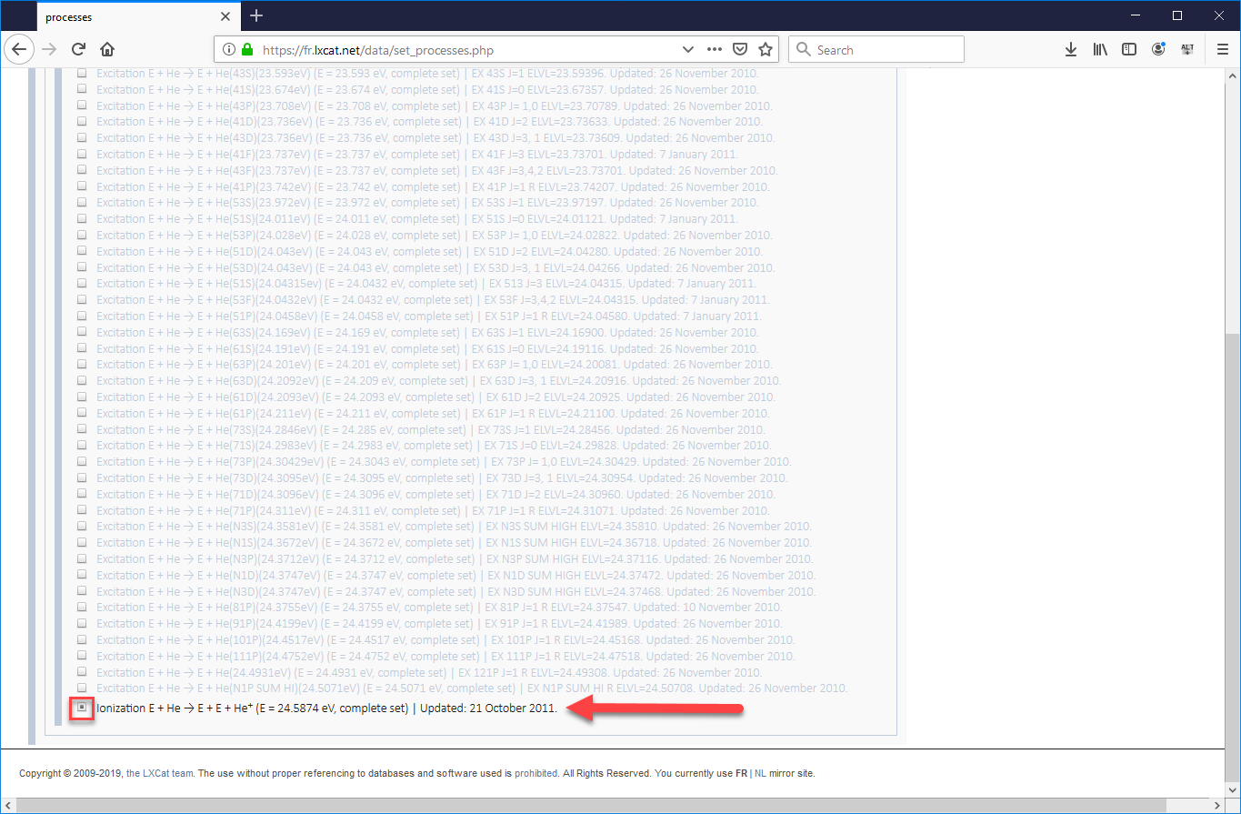
Fig. 543 LxCat Step 6b

7. This will take you to the Terms of Use page for the LxCat database. All the data in this database represents someone’s original research, and therefore must be appropriately cited when used in further research. Please read this page (it is very short), then press “Yes, I have read and understood >>” to proceed.

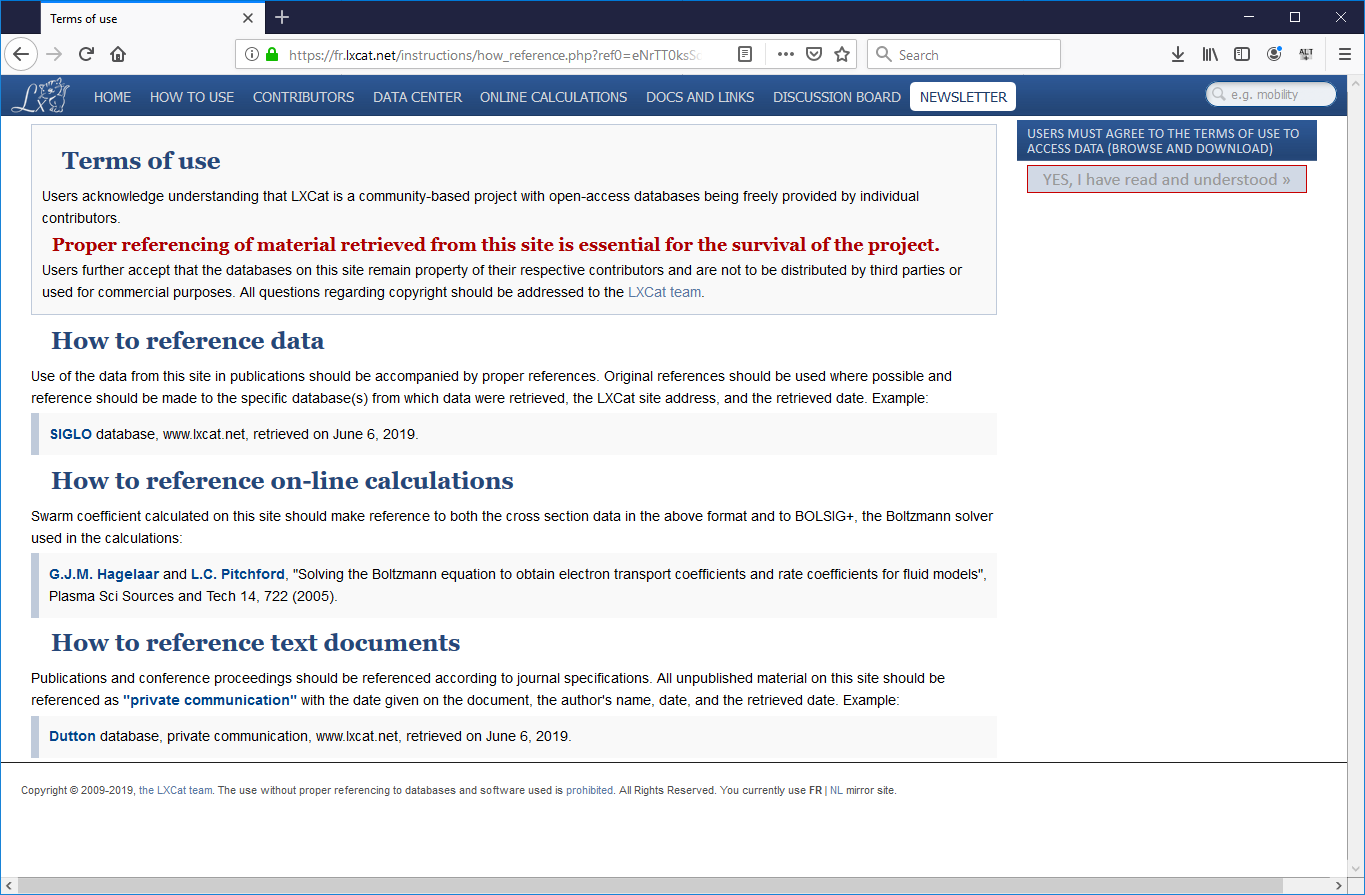
Fig. 544 LxCat Step 7

8. After agreeing to the terms of use, you will once again be shown the list of cross-sections from which you selected the 7 processes in Step 6. Just press “Next” one final time to retrieve the data.
9. On the next page there will be a plot showing the cross-section data you selected in Step 6. To use cross-section data in VSim, we need the data in a two-column format with no header. The two column need to have the CM energy (in eV) in the first column, and the cross section (in square meters) in the second column. To retrieve the data in this form, press the “TXT” text in the upper right corner (see Fig. 544).

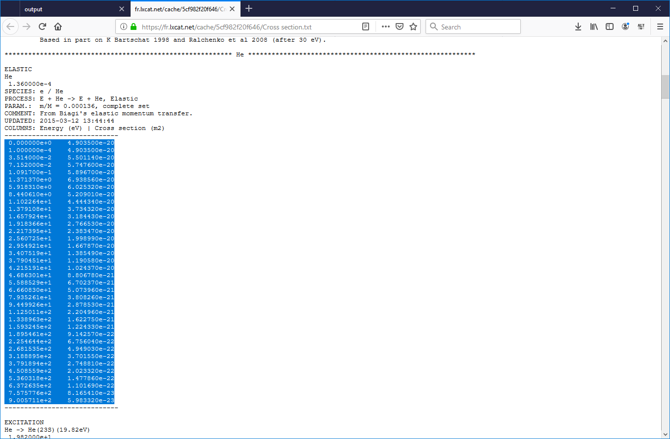
10. A new browser tab will open up. Scroll down past the headers to find the data. Notice that in the headers for each of the data sets, the units of each of the columns are given. This data happens to be in the correct units. Not all the cross-section data on the LxCat site is in eV and square meters.

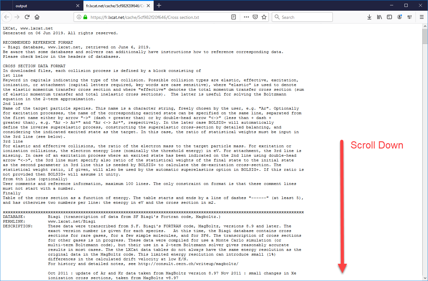
11. Highlight the data for one set, and copy it into a .dat file. Be sure to only select the data and no headers or other characters. The best way to create a .dat file is to copy the data into a .txt file, then change the .txt extension with .dat. This can be done in a Windows file browser.

12. Each of the seven data sets will need to be copied into their own .dat file, with the appropriate name. The name will need to match the string in the cross-section data file field of the particle reaction that uses the data set. This is how to import cross-section into collision processes that use the Reactions framework. For use with older frameworks like the Monte Carlo or Impact Collider frameworks, consult the appropriate documentation.

Running the Simulation

To run the simulation:

• Proceed to the run window by pressing the Run button in the left column of buttons.
• Here you can set run parameters, including how many cores to run with (under the MPI tab).
• When you are finished setting run parameters, click on the Run button in the upper left corner. You will see the output of the run in the right pane. The run has completed when you see the output, “Engine completed successfully.” This is shown in Fig. 548.

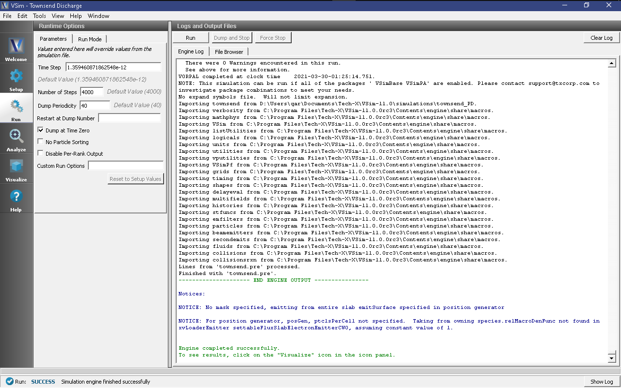
Fig. 548 The Run window at the end of execution.

Computing the Townsend Coefficient

To collect enough data and make a fit to

this simulation will need to be run multiple times with different plate separations. Since the electric field is constant, different plate separations correspond to different voltage differences between the right and left plates. As the plates get further apart, electrons will have more space to accelerate and ionize the neutral helium gas. Since the total number of helium ions created in collisions with electrons depends on the total number of electrons in the space between the two electrodes, the exponential form of the equation above is expected.

To adjust the plate separation, change the voltageDifference constant which is under Constants in the setup tree. The simulation will open with this constant set to 40 volts. When we performed this study, we ran at voltage of 40, 50, 60, 70, 80, 90, and 100 volt differences, then ran a least squares fit of the data to the shifted exponential in Mathematica. Our code for performing the fit is below:

In[1]:= Clear["Global`*"];

(* number of electrons *)
In[2]:= Ne = 100000
Out[2]= 100000

(*  number of ions from various runs *)
In[3]:= Ni = {5460, 13258, 22548, 33778, 46605, 60772, 77181}
Out[3]= {5460, 13258, 22548, 33778, 46605, 60772, 77181}

(* corresponding voltages *)
In[4]:= Voltage = {40, 50, 60, 70, 80, 90, 100}
Out[4]= {40, 50, 60, 70, 80, 90, 100}

(* distance increment corresponding to 10 volts *)
In[5]:= dL = 1/21200.
Out[5]= 0.0000471698

(* plate separations *)
In[6]:= Lvals = Voltage/10*dL
Out[6]= {0.000188679, 0.000235849, 0.000283019, 0.000330189, \
0.000377358, 0.000424528, 0.000471698}

(* Current ratio (measured/initial - for Nate's simulations, we will \
just define this directly from the data instead of computing from Ne, \
Ni *)
In[7]:= Ivals = N[1 + 2*Ni/Ne]
Out[7]= {1.1092, 1.26516, 1.45096, 1.67556, 1.9321, 2.21544, 2.54362}

(* Deviation from exponential growth *)
In[8]:= S = Total[(Log[Ivals] - m*Lvals - b)^2]
Out[8]= (0.933588 - b - 0.000471698 m)^2 + (0.795451 - b -
   0.000424528 m)^2 + (0.658607 - b - 0.000377358 m)^2 + (0.516147 -
   b - 0.000330189 m)^2 + (0.372225 - b -
   0.000283019 m)^2 + (0.235199 - b - 0.000235849 m)^2 + (0.103639 -
   b - 0.000188679 m)^2

(* Minimize with respect to m and b *)
In[9]:= mval = Expand[m /. Solve[D[S, m] == 0, m][[1]]]
Out[9]= 1668.61 - 2800. b

In[10]:= bval = Expand[b /. Solve[D[S, b] == 0, b][[1]]]
Out[10]= 0.516408 - 0.000330189 m

In[11]:= sols = Solve[{m == mval, b == bval}, {m, b}][[1]]
Out[11]= {m -> 2950.38, b -> -0.457775}

(* Predicted Townsend *)
In[12]:= AlphaTownsend = m /. sols
Out[12]= 2950.38

(* Predicted Alpha/p0 *)
In[13]:= AlphaTownsend/21.2/100
Out[13]= 1.39169

The In[3]:= line contains a list of helium ions counts collected from the 7 runs at different voltages, and correspond to the voltages in the list on the In[4]:= line. Plate separations are calculated based on the voltages in the In[6]:= line and are values for the independent variable, \(x_0\) in the equation to which we are fitting.

In the In[7]:= line we calculate an estimate for the total current that would be measured should the discharge be sustained continuously. We consider each particle to represent one “unit” of current. Therefore, the total current will be \(N_0 + N_{e,i} + N_{He,i}\) where \(N_0\) is the initial number of electrons emitted from the cathode, \(N_{e,i}\) is the number of electrons created in ionization collisions, and \(N_{He,i}\) is the number of helium ions created in collisions. Since math:N_{e,i} = N_{He,i}, ie the number of electrons created through collisions are the same as the number of helium ions created in collisions, we calculate the normalized current (quantity on the left side of the equation above) through the chamber here. The rest of the lines are performing the mathematics of the fit.

To obtain the data used on the In[3]:= line, follow these instructions:

1. After a simulation has finished running, proceed to the Visualize Window by pressing the Visualize button in the navigation column.
2. From the Add a Data View menu at the top left of the Visualize Window choose History. A new tab will open in which you can visualize data collected every timestep.
3. Set the history in Graph 1 to “numPhysHeIons” and set the other three Graphs to “None”. When the data is finished loading, your screen should look like the image in Fig. 549.

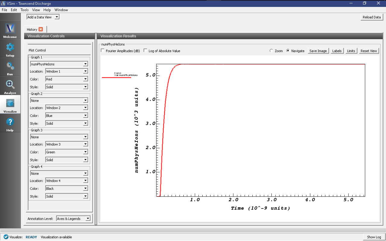
Fig. 549 The total number of helium ions in the simulation as a function of time.

4. Zoom into the end section of the plot to easily read off the total number of helium ions at the end of the simulation. An astute user might notice that some helium ions are absorbed while the simulation is running, so the number of helium ions isn’t an exact measure of the number of ionization events that occurred. To get the number of ions absorbed during the simulation, one can plot the HeUpperXAbsorbedCurrent and HeLowerXAbsorbedCurrent histories, where each spike in the histories represent the absorption of one ion. Since the total number of absorbed ions is around a percent of total ions, this isn’t a terrible approximation.

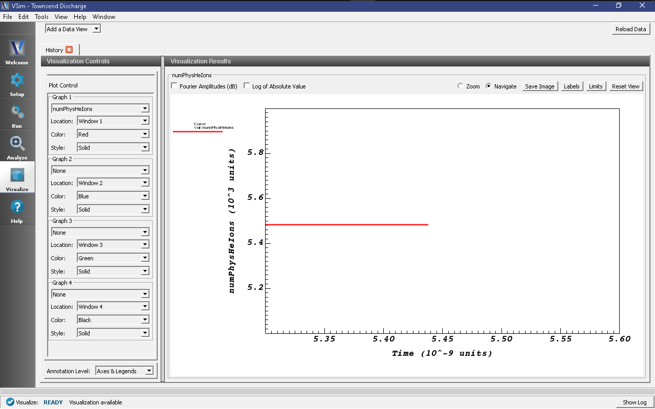
Fig. 550 A zoomed in view of the helium ion count at the end of the simulation.

5. Copy this value into the Mathematica (or whichever program you choose to run the fitting).

Further Experiments

1. Run the simulation at a different pressure to measure the Townsend coefficient in a different regime.
2. Change the gas type by switching the ion species, gas species, and cross-sections.