Turner Case 2 (Turner.sdf)

Problem Description

In this example we demonstrate VSim’s ability to simulate capacitively coupled plasmas, using the benchmark cases of Turner et al. [TDD+13]. Turner’s work documents the successful benchmarking of five independently developed particle-in-cell codes (not including VSim) for four different capacitive coupling scenarios at various background pressures.

Here, we consider the second of the Turner scenarios, though the input file can be readily modified to simulate the others. In addition to being able to accurately reproduce the Turner results, VSim can also employ physics-based initialization methods to enable more rapid convergence of the simulations to their steady-state. The use of such methods will also be explained below.

This simulation can be performed with a VSimPD license.

Opening the Simulation

The Turner example is accessed from within VSimComposer by the following actions:

• Select the New → From Example… menu item from the File menu.
• In the resulting Examples window expand the VSim for Plasma Discharges option.
• Expand the Capacitvely Coupled Plasmas option.
• Select Turner Case 2 and press the Choose button.
• In the resulting dialog, create a New Folder if desired, and press the Save button to create a copy of this example.

All of the properties and values that create the simulation are now available in the Setup Window as shown in Fig. 486. In this image, we have unclicked the electrons’ particleLoaderE and the HeNeutralFluid so that they will not hide the basic grid. You can expand the tree elements and navigate through the various properties, making any changes you desire. The right pane shows a 3D view of the geometry, if any, as well as the grid, if actively shown. To show or hide the grid, expand the Grid element and select or deselect the box next to Grid. This is a one-dimensional problem, which is shown by having the grid have only a single cell above and below the x-axis.

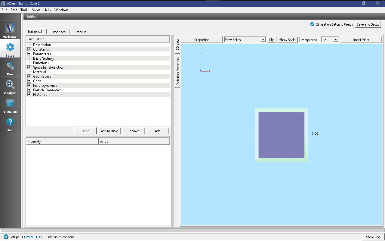
Fig. 486 Setup Window for the Turner example.

Clicking the electrons’ particleLoaderE shows that the electron loader is defined to exist over a cartesian 3d slab, even though this is a one-dimensional simulation. The dimensions that do not apply are ignored, with the coordinate set to zero, but this allows easy conversion from a 1D simulation to a 2D simulation.

Simulation Properties

The basic physics of this simulation is a balance between collisional processes and wall losses; a one-dimensional box of length 6.7 cm contains neutral helium gas at room temperature (300 K) and density 3.21e21/m^3 (1 Torr of pressure at that temperature). The gas is weakly ionized, resulting in a population of free electrons and singly ionized helium atoms at density 5.12e14/m^3. The helium ions are also at room temperature, while the electrons are considerably hotter (30,000 K). The left wall of the box is grounded, while the right wall oscillates with a bias voltage of 200 V at frequency 13.56 MHz.

Charged particles are lost upon collision with the wall and are replenished by ionization of the background neutral gas by the hot electrons; the latter process repopulates both the electrons and helium ions in the plasma (the background neutral gas is treated as an infinite source). Plasma sheaths form near the walls, containing electric fields which are strong relative to those elsewhere in the plasma; the particle density profiles adjust in response to the fields in the sheath. The sheath transit time, for ions, is much longer than the period of the oscillating potential; thus, multiple RF cycles occur while an ion crosses the sheath. A steady state is attained when the loss rate of particles to the wall comes into balance with the ionization rate for a particular profile shape.

In our initial run we are not going to model the full evolution of the discharge to its steady-state parameters; rather, we will explore the basic physics of the discharge and modify the simulation accordingly (with the aim of ultimately hastening convergence to this steady state, while exploring VSim capabilities).

Running the Simulation

The original runs by Turner were for about 4,000,000 steps. However, the asymptotic state is reached after about 300,000 steps. To illustrate how to run this problem, we will run for only 10,000 steps, which takes about 5 minutes on a 4-core i7 Windows workstation.

To run the simulation, continue as follows:

• Proceed to the Run Window by pressing the Run button in the left column of buttons.
• Select the ‘Run Mode’ drop down menu and change it to parallel.
• Set ‘Number of Processes’ corresponding to your VSim license, shown above as the ‘Licensed Cores’
• To run the file, click on the Run button in the upper left corner of the window. You will see the output of the run in the right pane. The run has completed when you see the output, “Engine completed successfully.” A snapshot of the simulation run during execution is shown in Fig. 487.

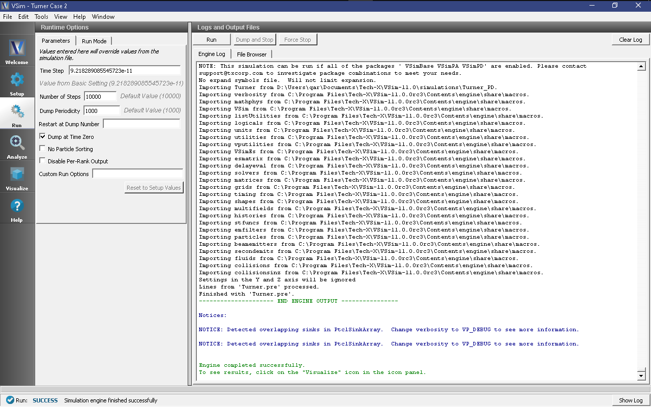
Fig. 487 The Run Window during execution.

Analyzing the Results

We are going to run a postprocessing script, computePtclNumDensity.py, which builds density profiles from the particle data generated by VSim, so that we can look at these profiles and their evolution. To do so, we do the following:

• Click the Analyze beneath the run button in the leftmost pane.
• From the Available Analyzers, choose computePtclNumDensity.py. Then click Open.
• Fill in the text boxes
  • The simulationName should be already filled in, but if it is not, type in the name of the .sdf file without the .sdf extension.
  • For the speciesName, type in ‘electrons’ without the quotes.
• Click Analyze (in the Analyze Window); this will generate the electron density profiles.
• Now replace ‘electrons’ in the speciesName box with ‘He1’, for the helium ions.
• Click Analyze (again in the Analyze Window) to generate the ion density profiles.
• The name of the resulting data is electronDensity and He1Density, which will be visualized in the next section.

Visualizing the Results

Now that we have all of our data, let’s look at it.

• Click the Visualize button beneath the Analyze button in the leftmost pane.

After a brief moment the visualization options for this data should appear.

We will first look at the time evolution of some fundamental one-dimensional quantities. From the Add a Data View pulldown menu on the top left, select History. The default view here should contain four plots, namely, the electron and ion currents to the left wall and the number of electron and ion macroparticles in the simulation. A number of notable physics effects can be seen here:

• After a sharp initial decrease in the electron population, both ion and electron populations decline at approximately the same rate. This is not as apparent from the separate numElec and numIons plots, but with some selection of the plot controls we can combine and reduce the number of plots. In Graph1, select “numElec” as the variable to plot and select “Black” as the color. In Graph 2, select “numIons” to plot, “Window 1” as the Location, and “Green” as the color. In Graph 3 and Graph 4, select “None” as the variable to plot. This should produce the view seen in Fig. 488. The initial decrease in electron population arises when rapid electron wall losses create a charge imbalance in the plasma and establish plasma sheaths near the walls. Thereafter, this charge imbalance is preserved and the transport of both electrons and ions to the wall becomes ambipolar.

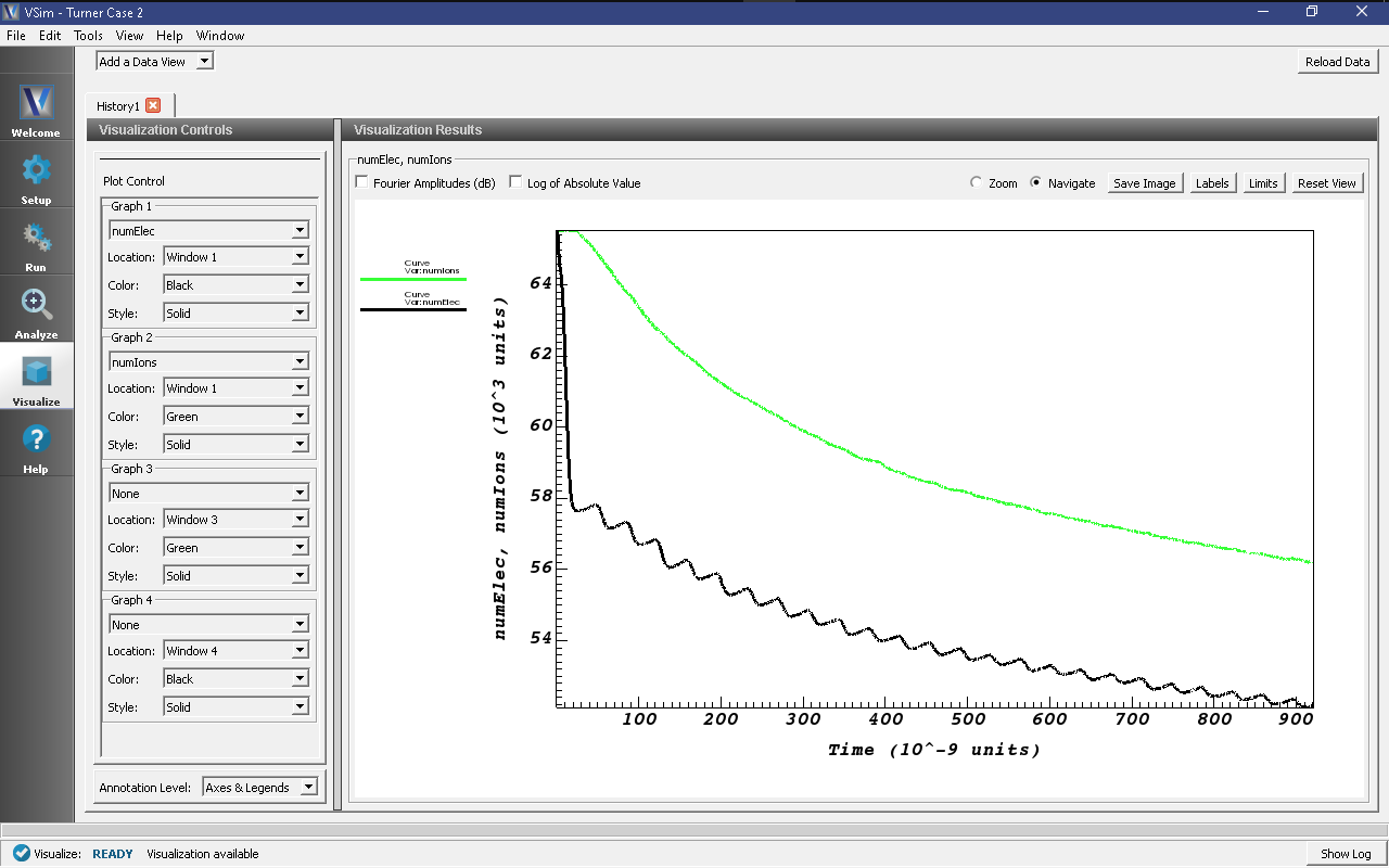
Fig. 488 The electron and ion populations versus time.

• The electron wall currents are quasi-periodic. The oscillating potential drives the highly mobile electrons alternately into the left and right walls. In the plot variable menu, change “numElec” to “leftElecCurr” in Graph 1 and “numIons” to “rightElecCurr” in Graph 2. The impacts of the electron cloud on the left and right walls, and their phasing in time, can be seen in response to the potential oscillations. A history of the electron currents can be seen in Fig. 489

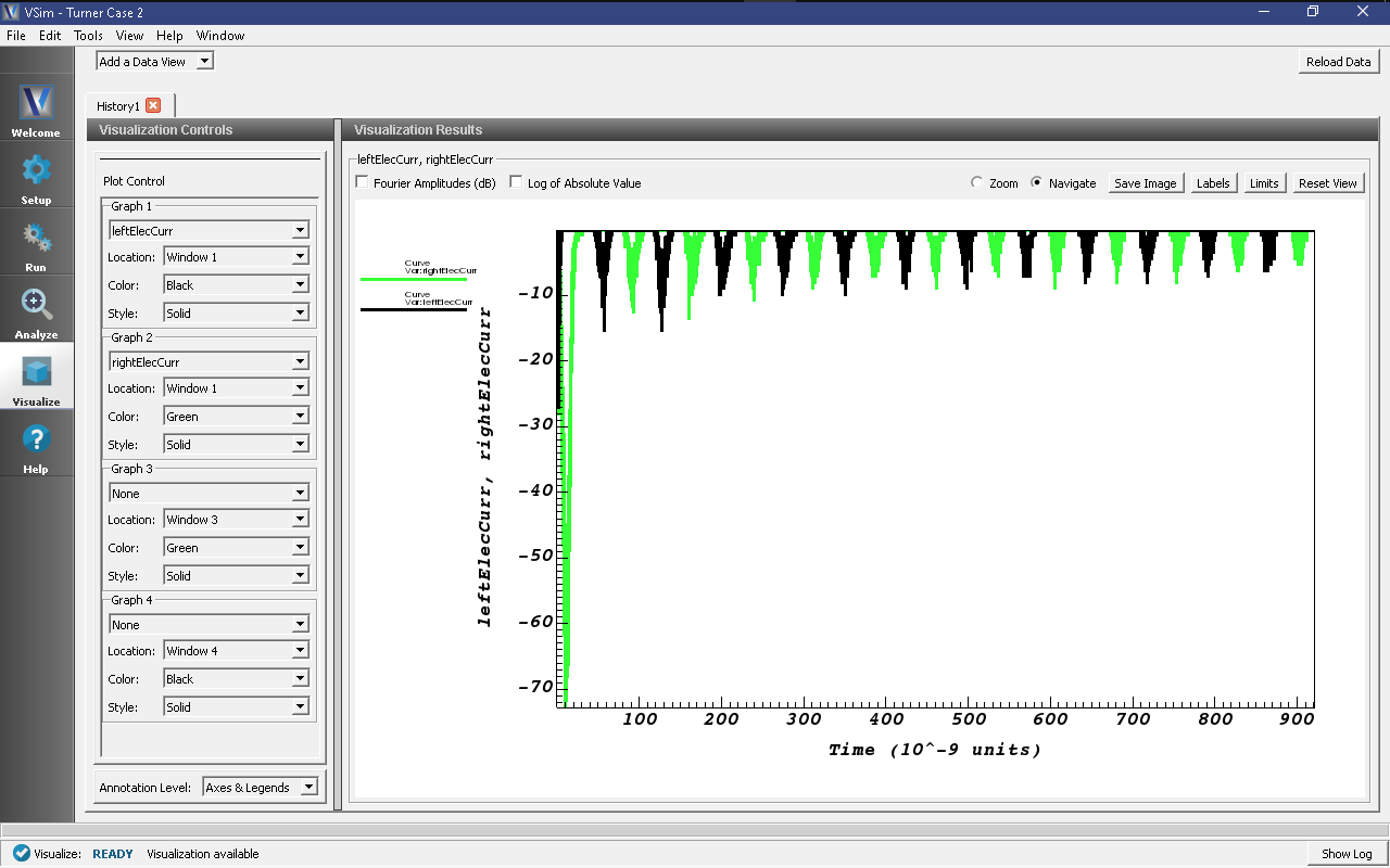
Fig. 489 Electron currents on the left (black) and right (green) walls versus time

• The ion currents are non-periodic. Ions, being much heavier than the electrons, exhibit relatively little response to the oscillating potentials. In the plot variable menu, change the Graph 3 quantity “None” to “leftIonCurrent” and the location to “Window 1”, then change the Graph 4 quantity “None” to “rightIonCurrent” and the location again to “Window 1”. The ion currents do not have the quasi-periodic structure of the electron currents; rather, ions diffuse outward to the walls in response to the DC sheath potentials, which are established by the initial departure of electrons and may also be rectified by the RF. A history of all the particle currents can be seen in Fig. 490

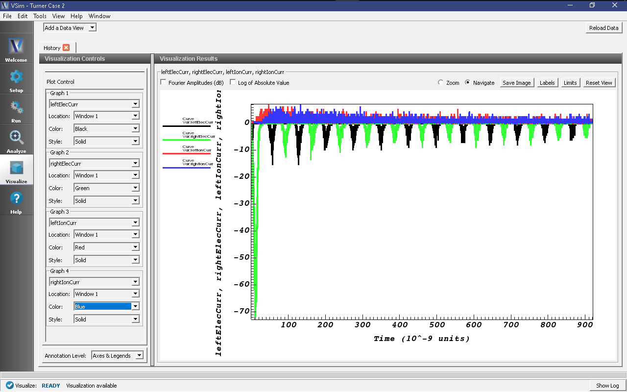
Fig. 490 Electron and ion currents on the left and right walls versus time

• Ion losses are negligible before the initial establishment of the sheath. Change the plot quantity in Graph 3 from “leftElecCurr” to “None”. Change the plot quantity in Graph 4 from “rightElecCurr” to “numElec” and for the first two graphs change the “Location” to “Window 3”. It is clear that the dominant loss of ions to the wall only begins after the initial decrease in electron population (which corresponds to the establishment of the sheath). A history of the electron population against the ion currents can be seen in Fig. 491

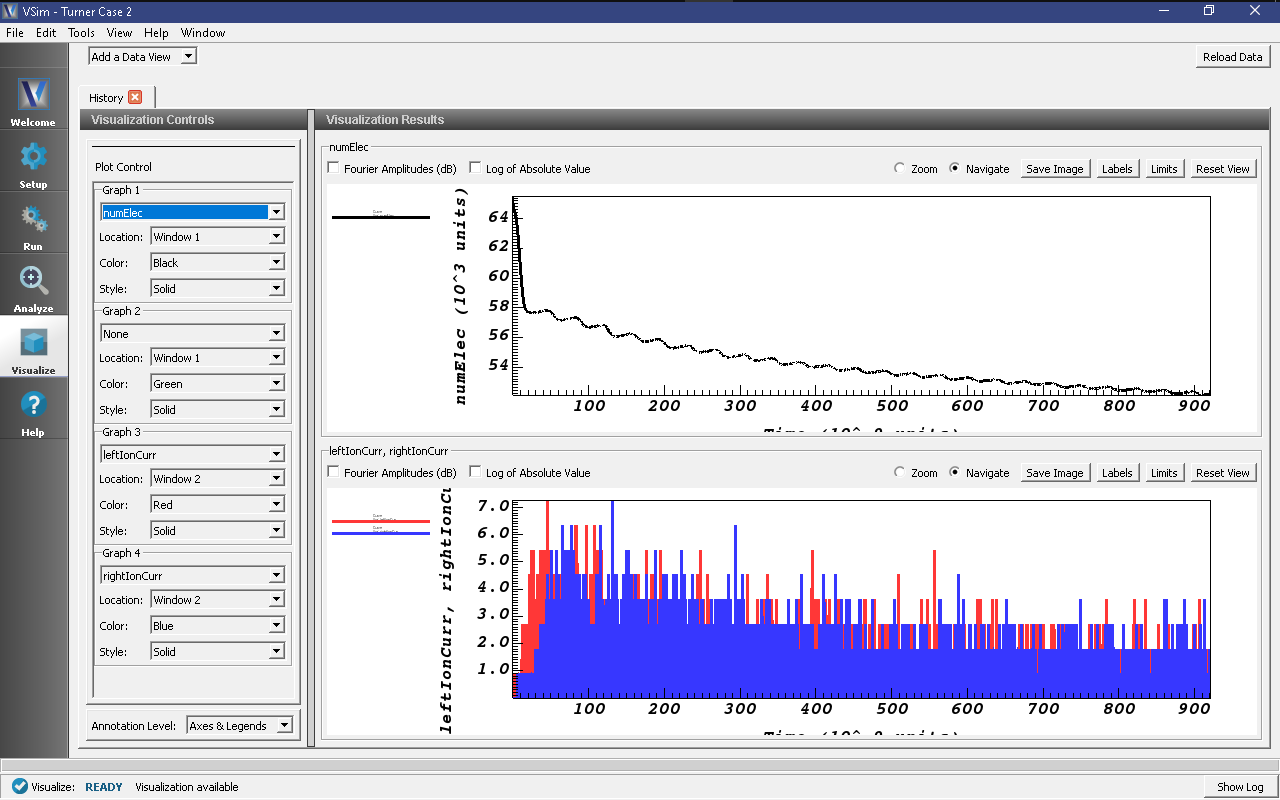
Fig. 491 History plots showing the majority of the ion current to the walls only begins after initial decrease in electron population

We can also look at the plasma sheath and the ensuing changes in density profiles directly. In the “Add a Data View” menu at the top left of the Composer window, select “1-D fields”. The plot controls here are similar to those of the history window. Select “E_x” for the plot variable in Graph 1. Select “Phi” for the plot variable in Graph 2. Select “electronsDensity” for the plot variable in Graph 3. Select “He1Density” for the plot variable in Graph 4, and select “Window 3” for the location of this plot. The evolution of the discharge in time can be viewed by moving the time slider below the plots. Slide the bar to dump 10 to view the data at time step 10000 (the data was saved every 1000 time steps).

A number of additional physics features can be seen:

• Sheath effects are present. Regions of sharp potential variation, corresponding to strong electric fields, arise near the walls, but such fields are screened out in the bulk plasma. Moving the time slider, it is clear that this sheath behavior persists regardless of the phase of the oscillating wall potential.
• Electron profiles are altered much faster than ion profiles. Both ions and electron profiles are initially constant (5.12e14 1/m^3), but by the time the first nontrivial dump file is produced (at time dumpPeriodicity * dt, approximately 1/3 of the way through the period of the first wall oscillation), electron-poor regions corresponding to the sheaths have already been established in the electron profile, while the ions have barely begun to respond to the presence of the sheath. Moving the slider forward in time, one observes that the electron profile predominantly oscillates in response to the wall potential, while the ion profile evolves considerably more slowly, particularly outside the sheath regions. The 1-D fields at time step 10000 (dump 10) can be seen in Fig. 492

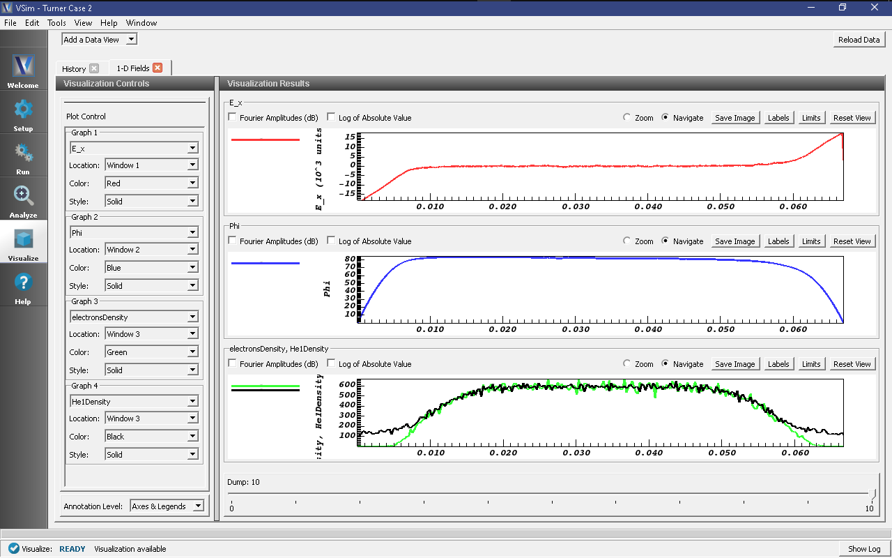
Fig. 492 Plots of various 1-D field quantities showing the final state of the run at time step 10000.

Further Experiments

Now that we understand some of the basic physics of the discharge, we are in position to apply physics-based particle loading methods to hasten its eventual convergence to steady-state. The underlying principle here is to identify the ‘slow’ processes involved in the evolution of the discharge toward steady state, and then alter the loading to more closely mimic the state to which the plasma is being driven. While we cannot entirely predict the parameters of the steady-state, it is not difficult to at least get some idea of how the simulation is evolving and adjust the particle loads accordingly. We have already observed a number of physical processes of possible relevance:

• initial electron loss and the establishment of ambipolarity
• the slow decay of the total ion and electron population following the initial electron loss
• the rapid response of electrons to applied electric fields, particularly in the sheath region
• the slow evolution of ion density profiles.

Of these, we will primarily consider the ion profiles; the high mobility of the electrons suggests that electron profiles will adjust correspondingly on much shorter timescales. Additionally, since the strong electric fields in the plasma sheath region are screened out via Debye shielding as we move away from the walls, it seems clear that profile adjustments in the bulk plasma (where the driving electric fields are weakest) will ensue more slowly than in the plasma edge. We therefore concentrate our attention first on obtaining an approximately correct value for the ion density at the center of the domain.

In the ‘1-D Fields’ tab, set the plot variable to ‘None’ in plots 2, 3, and 4. In Graph 1, set the plot variable to ‘He1Density’ and again move the timeslider on the bottom right of the window. The central ion density steadily rises; from its initial value of 5.12e14/m^3, it rises to 6e14/m^3 by the end of our comparatively short run. In addition, a rapid decrease in density near the walls (associated with the plasma sheath) has lowered the edge densities to about 1e14/m^3. The ion density can be seen in Fig. 493

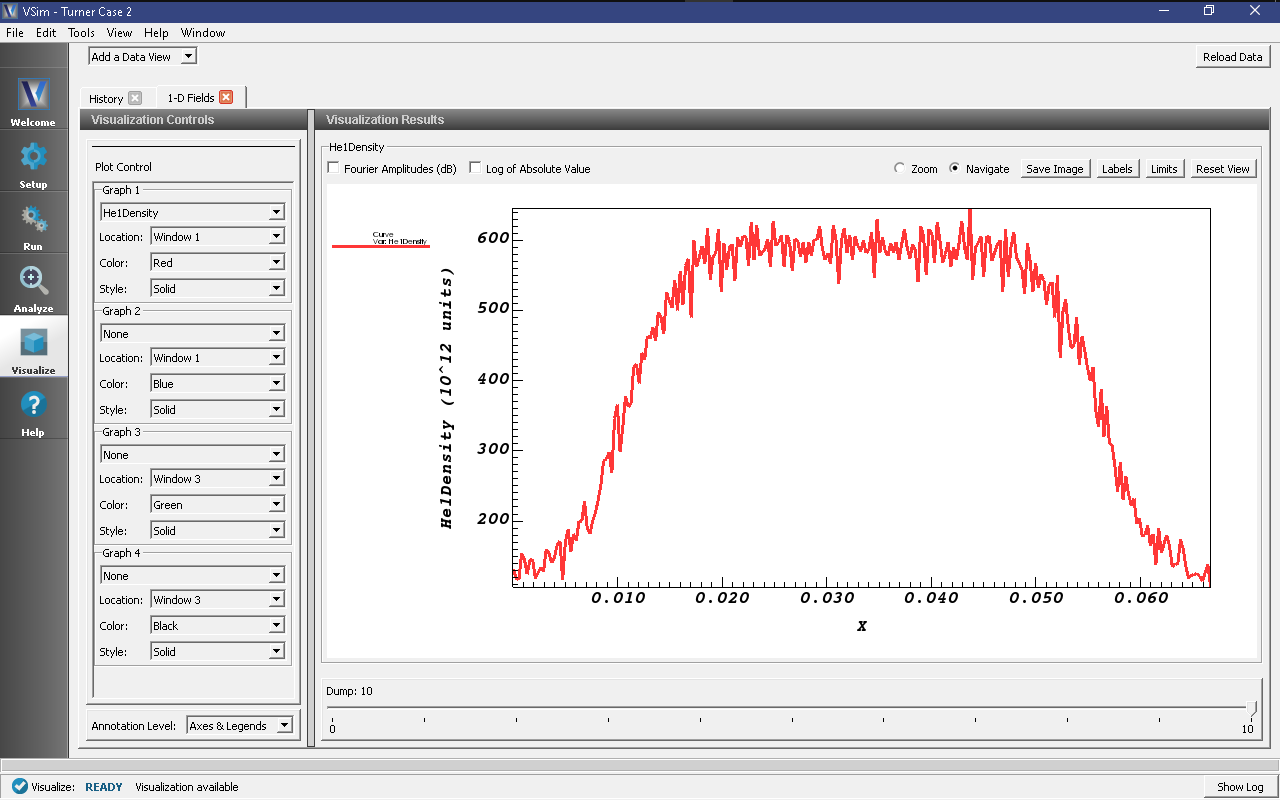
Fig. 493 The He ion density at the end of the run (time step 10000).

Additional Studies

It is possible to try other techniques to converge to steady state faster. These techniques are outlined in detail in the text-based version of this example. In summary:

Another thing you can try are by loading the particle with a non-uniform profile that better resembles the outcome.

Yet another is to leave a gap near the walls when loading electrons and ions. What happens in the discharge? The electrons, being highly mobile, rush to fill the gap, but rather than immediately being lost to the wall, they instead produce strong electric fields at the plasma edge which begin to modify the ion profile and bring about ambipolarity. If the gap is sufficiently large, the collisional production of ions and electrons will begin before appreciable wall losses ensue, and we can thus assess the relative rates of production and loss fairly early in the simulation. Since the electrons are highly mobile, let’s treat the average electron population as a measure of how well we’ve achieved this balance; net electron production as we move into the ambipolar phase means that our gap is too low (we have removed too much density), while net losses mean that our gap is insufficiently wide. As the profile shapes near the walls tend to adjust themselves fairly quickly (due to the larger electric fields in this region), we can in this manner obtain approximately correct values for the total ion and electron populations at the simulation outset.