Multistage Collector (multistageCollector.sdf)
Keywords:
-
electromagnetics, multistageCollector
Problem description
Multistage Depressed Collectors (MDCs) are used to recover energy from a spent beam in linear type microwave tubes such as traveling wave tubes (TWTs) and klystrons. VSim provides the capability to simulate these collectors shaped with arbitrarily complex geometries and depressed with different time-dependent voltage profiles to optimize the recovery efficiency of a design. To demonstrate this capability, we show in this example a 4-stage depressed collector. One can adjust the depressed potentials at each electrode individually to see how the performance of the collector is affected.
This simulation can be performed with a VSimMD or VSimPD license.
Opening the Simulation
The Multistage Collector example is accessed from within VSimComposer by the following actions:
- Select the New → From Example… menu item in the File menu.
- In the resulting Examples window expand the VSim for Microwave Devices option.
- Expand the Other MD option.
- Select “Multistage Collector” and press the Choose button.
- In the resulting dialog, create a New Folder if desired, and press the Save button to create a copy of this example.
The Setup Window is now shown with all the implemented physics and geometries, if applicable. See Fig. 452.
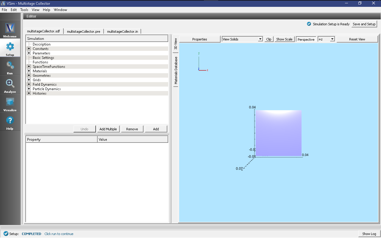
Fig. 452 Setup Window for the Multistage Collector example.
Simulation Properties
The simulation geometry consisting of an S-band 4-stage depressed collector is imported into the computational engine from CAD files in stl format. One can easily create new geometry using any CAD program and output or convert the CAD files into stl files for a new simulation design. The detailed import method is provided in the input file. The spent beam profile is taken from a TWT simulation provided by Prof. H. Song at University of Colorado at Colorado Springs.
An optimized design for a MPM module can be found in reference [1]. Users can set preferred spent beam profiles by employing different emission methods or import data in dat format as in this example. A main feature of this input file is that the depressed voltage profiles are time-dependent and are stabilized with a new external circuit model based on special feedback algorithms only available in VSim. Interested users may refer to the publication for more a detailed description and validation. In addition, the convergence of this example is carefully tested.
In this example, the Z coordinate is the direction aligned with the beam axis of the MDC, and the 4 different voltages can be easily assigned at the input panel. Since it is a time domain simulation, the Dey-Mittra algorithm is employed and the accuracy is second-order for the complex boundaries.
Running the simulation
After performing the above actions, continue as follows:
- Proceed to the run window by pressing the Run button in the left column of buttons.
- To run the file, click on the Run button in the upper left corner of the right panel. You will see the output of the run in the right pane. The run has completed when you see the output, “Engine completed successfully.” This is shown in Fig. 453.
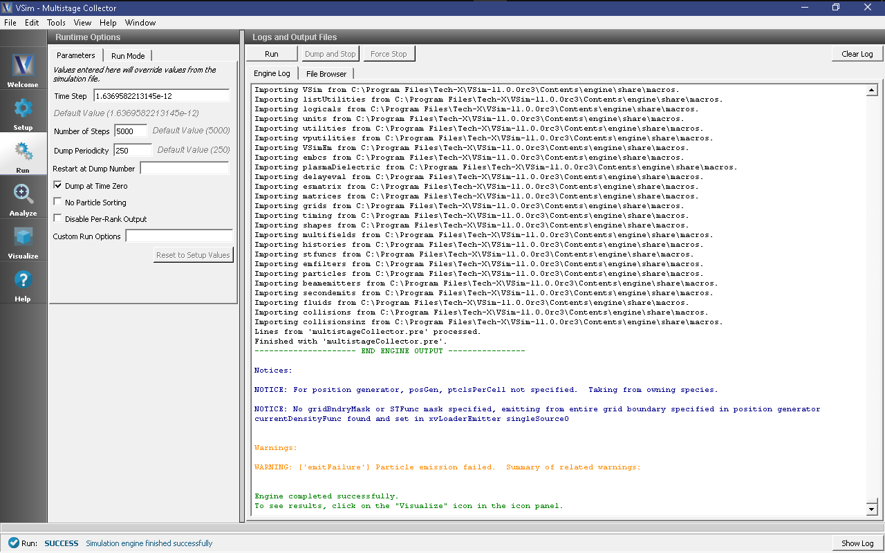
Fig. 453 The Run Window at the end of execution.
Visualizing the results
After performing the above actions, continue as follows:
- Proceed to the Visualize Window by pressing the Visualize button in the left column of buttons.
The results are then read from the Data Overview in the Visualize Window:
- Expand Particle Data.
- Expand electrons.
- Select electrons in red.
- Check the Clip Plot box.
- Click on Plane Controls and in the Clip Plane Control window, under Clip Plane Normal select X (plane normal to x-axis), then click Ok.
- Expand Scalar Data.
- Expand E.
- Select E_z.
- Check the Display Contours box.
- Check the Clip Plot box.
- Click on Plane Controls and in the Clip Plane Control window, under Clip Plane Normal select X (plane normal to x-axis), then click Ok.
- Expand Geometries
- Select the second option from the top: multistageCollectorGeomSolidMappedPolysData_surface.
- Check the Clip Plot box.
- Click on Plane Controls and in the Clip Plane Control window, under Clip Plane Normal select X (plane normal to x-axis), then click Ok.
- Move the Dump slider all the way to the end.
- Use the cursor to grab the image and rotate it from right to left to see the image in Fig. 454.
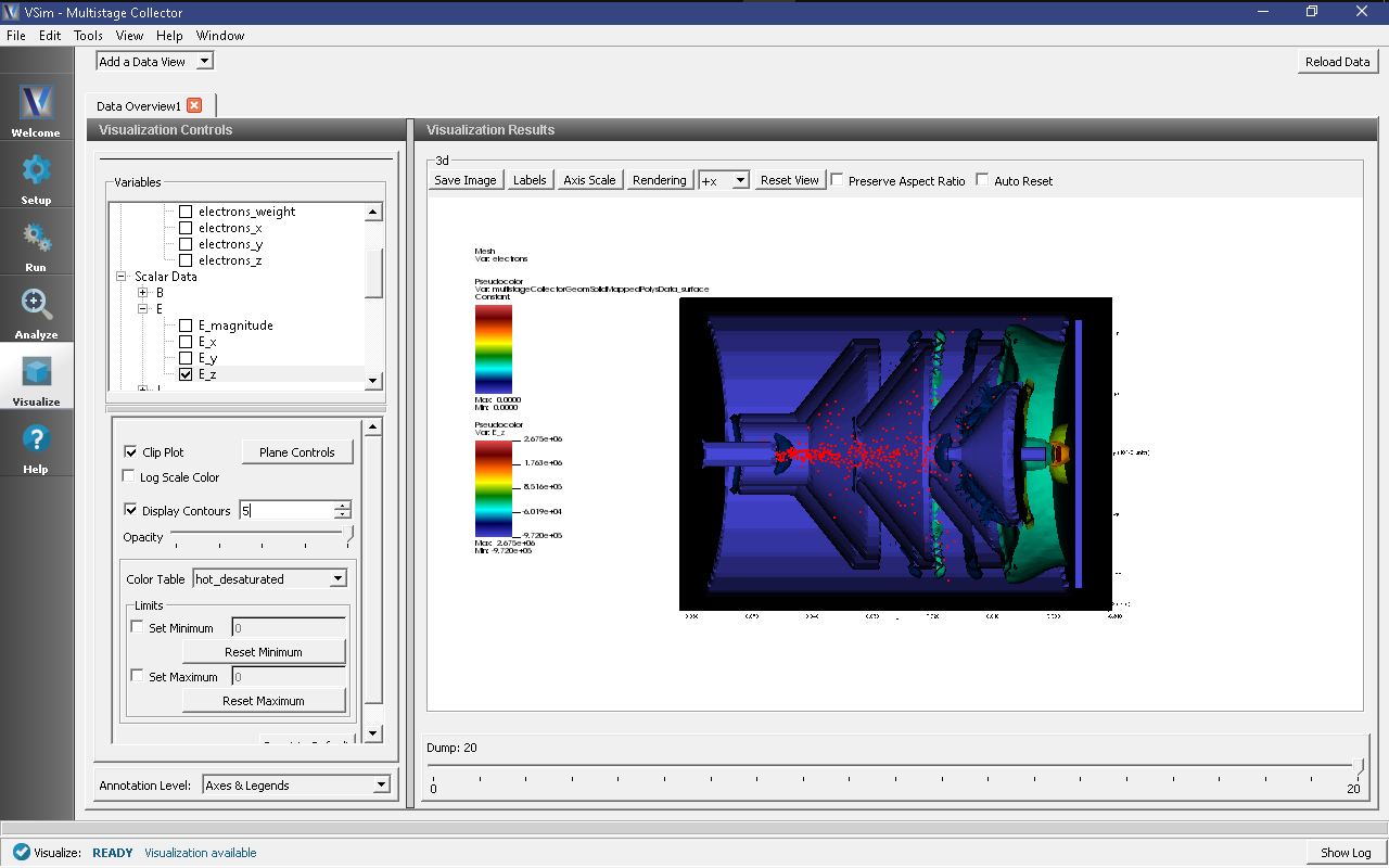
Fig. 454 Visualization of the MDC model with a color contour plot of electric fields and electrons in red.
The potential of each of collector surfaces is recorded using a history. To visualize these values as shown in Fig. 455, do the following:
- Switch Data View to “History”.
- In the left pane, set Graphs 1-4 to each of the different potential histories: “potential10”, “potential20”, “potential30”, and “potential40”, respectively.
- Set the Location of each graph to the “Window 1”.
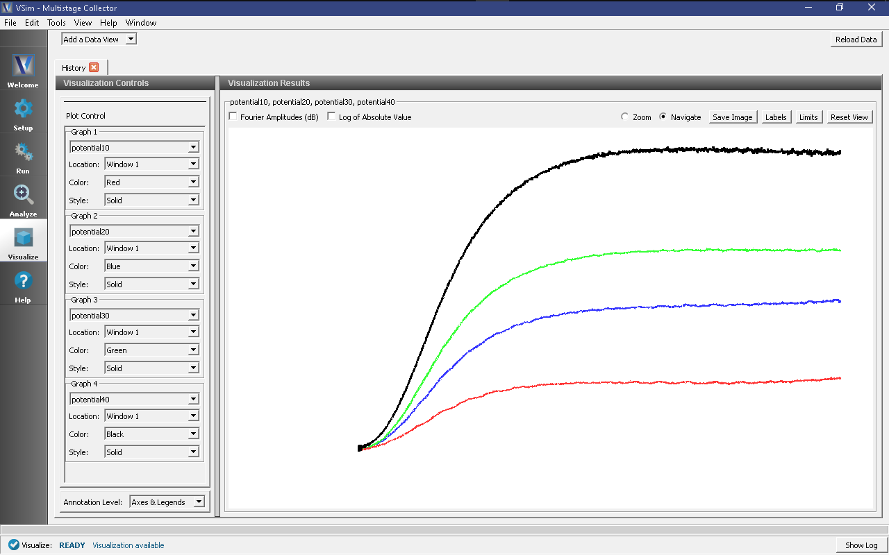
Fig. 455 The value of the potential on each of the collectors.
Further Experiments
The depressed voltages or beam current/radius can be varied in the input panel for testing runs. One can also change the grid cell numbers to see the convergence of the simulations.
References
- [1] M. C. Lin, P. H. Stoltz, D. N. Smithe, H. Song, H. J. Kim, J. J. Choi, S. J. Kim,
- and S. H. Jang, “Design and Modeling of Multistage Depressed Collectors Using 3D Conformal Finite-Difference Time-Domain Particle-In-Cell Simulations ”, J. Korean Phys. Soc. 60, 731-738 (2012).