Multimode Fiber with Mode Launcher (multiModeFiberModeLaunchT.pre)
Keywords:
-
Mode Loading, Photonic Waveguide, Unidirectional Mode Launcher, MAL, Guided Mode, Semiconductor
Problem Description
This example consists of a single, straight cylindrical fiber waveguide that is parallel to the x-axis and centered at the origin. The waveguide is surrounded by a background material with a greater permittivity. Matched Absorbing Layers (MALs) are used to dampen the E and B fields near the boundary of the simulation. This is a way to dampen reflected fields from the simulation boundaries.
The fundamental guided mode is launched in the waveguide. The fundamental mode was extracted in the “Multimode Fiber Mode Calculation” example using the computeDielectricModes.py analyzer. A sample mode comes with this example saved in the file save4Launch_EigenD_0.vsh5, but this can be replaced another mode from the mode calculation example if the user desires. We take the field profile from the save4Launch_EigenD_0.vsh5 file and then apply time dependence via a SpaceTimeFunction, timeCompSingleFrequency. By launching the true eigenmode into the waveguide we should minimize losses and see a constant field profile.
This simulation can be performed with a VSimEM license.
Opening the Simulation
This example can be accessed from within VSimComposer through the following steps:
- Select the New → From Example… menu item in the File menu.
- In the resulting Examples window, expand the VSim for Electromagnetics option.
- Expand the Photonics (text-based setup) option.
- Select Multimode Fiber with Mode Launcher (text-based setup) and press the Choose button.
- In the resulting dialog, create a New Folder if desired, and press the Save button to create a copy of this example.
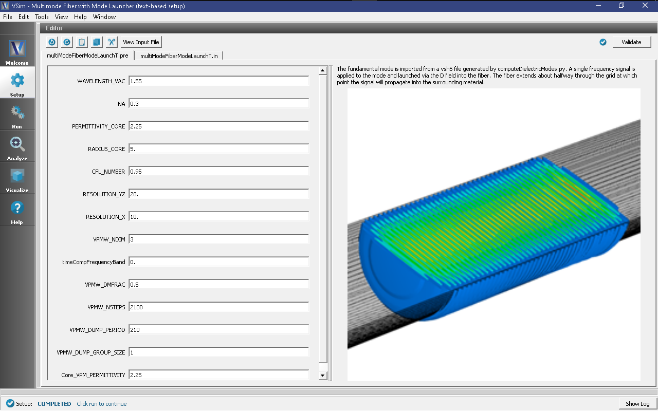
Some relevant parameters should now be visible as seen in Fig. 288.
Simulation Properties
This example contains a number of constants defined in the Multimode Fiber Mode Calculation example. These constants should not be modified if you wish to launch a true eigenmode. Some relevant constants that could be modified are listed below.
RESOLUTION_X: The number of cells per estimated wavelength in the propagation (x) direction.
CFL_NUMBER: The time step, DT, will be this value times the limit for numerical stability.
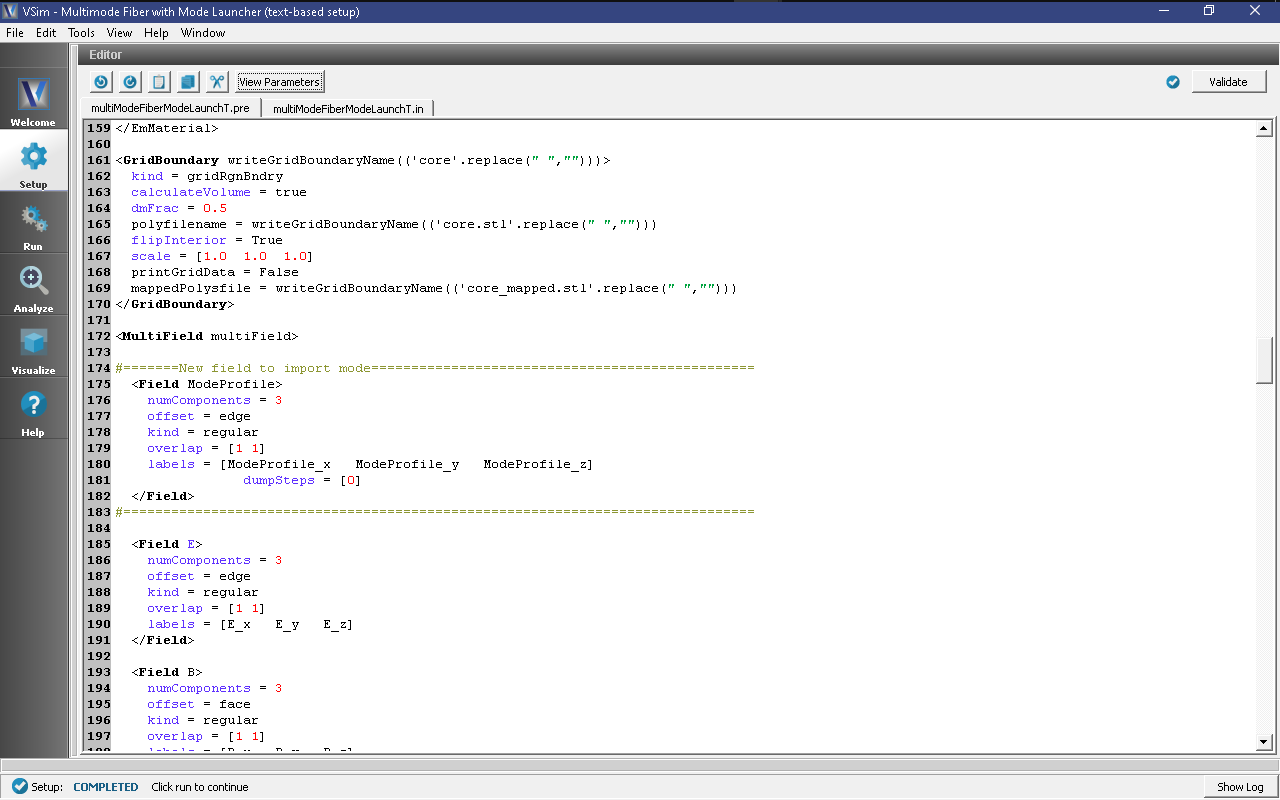
To expose more variables and see the geometries, boundary conditions, and fields, select View Input File. From here you can see the modifications made to import the eigenmode from the .vsh5 file. The modifications are clearly set apart with rows of equal signs as seen in Fig. 289.
The variables NBGNX_SOURCE, NENDX_SOURCE, NBGNYZ_SOURCE, and NENDYZ_SOURCE define where the source is located in integer grid cells. This should likely correspond to the location you specified when running the computeDielectricModes.py analyzer. To ensure the source is aligned with the fiber, we recommend using the same grid for mode extraction and mode launching and then defining the aforementioned variables as is seen in the input file.
The D field in the specified source location depends spatially on the imported mode and temporally on the expression timeCompSingleFrequency, which drives the mode at its respective frequency for a length of time, TIME_EXCITE. In photonics simulations, Matched Absorbing Layers (MALs) are the most stable boundary conditions for limiting reflections.
Running the Simulation
After performing the above actions, continue as follows:
- Proceed to the Run Window by pressing the Run button in the left column. You will be asked to Save. Click Save.
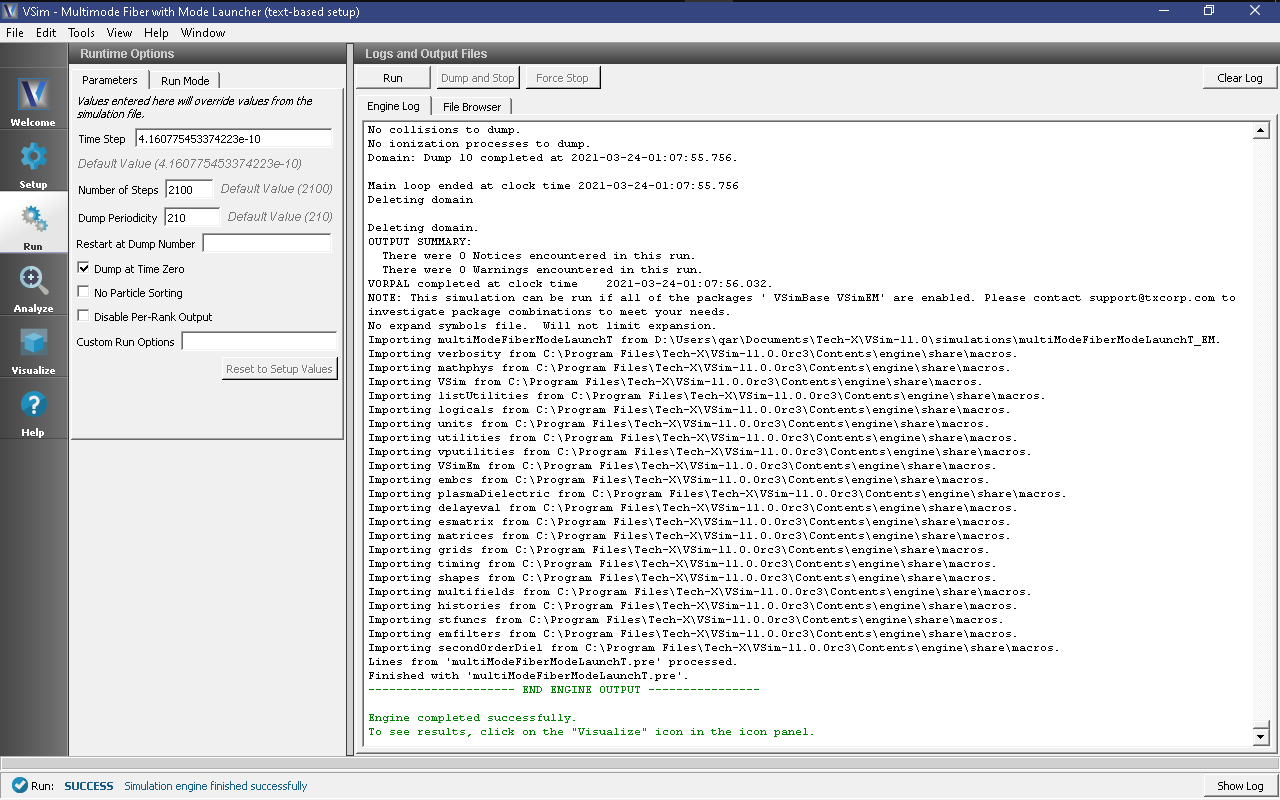
- To run the file, click on the Run button in the upper left corner of the right pane. You will see the output of the run in the right pane. The run has completed when you see the output, “Engine completed successfully.” The result is shown in Fig. 290.
Visualizing the Results
Then proceed to the Visualize window by pressing the Visualize button in the left column.
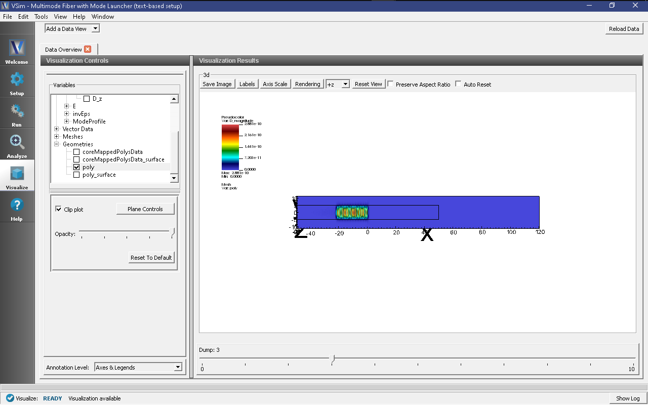
A useful visualization of the dielectric waveguide would be to view the magnitude of the D field to qualitatively see the mode propagate down the waveguide.
- Near the top left corner of the window, make sure Data View is set to Data Overview.
- Expand Scalar Data, expand D, and select D_magnitude
- Check the Clip Plot checkbox.
- Expand Geometries and select poly to show how far the waveguide extends.
- Once again, check the Clip Plot checkbox.
- Slide the Dump Slider (beneath the Visualization Results) to Dump 3
Your screen should resemble Fig. 291. Indeed, the mode launch is quite clean! To see what happens at the end of the fiber slide the dump slider further.
Further Experiments
One can experiment by changing constants or introducing a different signal to drive the waveguide and note the effects on loss or propagation.
One could also choose a different mode generated by the Multimode Fiber Mode Calculation example and launch that.


