Dielectric Waveguide with Dispersion (waveguideWithDispersion.sdf)
Keywords:
- Photonic Waveguide, Guided Mode, Waveguide Mode Solver, Dispersion, Dielectrics
Problem Description
This example simulates guided modes in dielectric waveguides (with and without dispersion), and highlights several XSim features: (1) the computeWaveguideModes.py analyzer, (2) 2nd-order dispersive dielectrics using the cut-cell Lorentz algorithm, and (3) launching waveguide-mode pulses into multiple waveguides. In the end, we will see how a weakly-dispersive material affects the group velocity of a mode in a cylindrical fiber.
The cylindrical waveguides in our simulation have axes in the x direction, and so eigenmodes take the form:
The effective index of refraction of a waveguide mode is given by \(\bar{n} = k / k_0\) where \(k_0 = \omega / c\). If the waveguide has index of refraction \(n_w\) and the cladding \(n_c < n_w\), then a guided mode will have a modal index in the range, \(n_c < \bar{n} < n_w\) (in our case, \(n_c=1\)).
The dispersion relation, \(\omega(k)\), of a waveguide mode determines the group velocity \(v_g\) of a pulse, which is approximated by \(v_g\approx\partial\omega/\partial k\). When the dielectric constant of the waveguide depends (weakly) on the frequency of the wave, we see a slight change in the slope of the dispersion relation \(\omega(k)\), and therefore a slight change in the propagation speed of a pulse.
We will demonstrate this change in group velocity using a few made-up materials in a custom vmat materials database file. The dispersive and non-dispersive materials will have a nearly identical dielectric constant at the working frequency (same phase velocity) but the dielectric constant of the dispersive material will have a weak frequency dependence.
The high-level overview of our workflow:
Set up the simulation (grid, waveguide geometries, and wave launchers).
Assign a non-dispersive dielectric constant (the dielectric constant at the working frequency) to each waveguide (the computeWaveguideModes.py analyzer does not yet support dispersive dielectrics; this is not an issue, however, since the analyzer is given a mode frequency as an input, and it is assumed the dispersive dielectric constant \(\varepsilon(\omega)\) can be sampled at the working frequency).
Run for 1 time step to generate finite difference matrices.
Run the computeWaveguideModes.py analyzer once for each waveguide cross-section.
Visualize the waveguide modes.
Assign the weakly-dispersive Lorentz dielectric material to one waveguide.
Assign the non-dispersive Lorentz dielectric material to the other waveguide.
Activate the mode launchers and run the simulation for many timesteps.
Visualize pulses propagating at different speeds in each waveguide despite matching phase velocities.
This simulation can be performed with a XSimEM license.
Opening the Simulation
In XSimComposer,
Select the New → From Example… menu item in the File menu.
In the resulting Examples window expand the XSim for Electromagnetics option.
Expand the Photonics option.
Select Waveguide with Dispersion and press the Choose button.
In the resulting dialog, create a New Folder if desired, and press the Save button to create a copy of this example.
You should see a setup screen like Fig. 287. As provided, the simulation is set up for the waveguide mode solver process (i.e. the mode launchers are turned off and the waveguide cylinders have been assigned a non-dispersive dielectric constant). Before running any tasks, we briefly discuss the simulation setup.
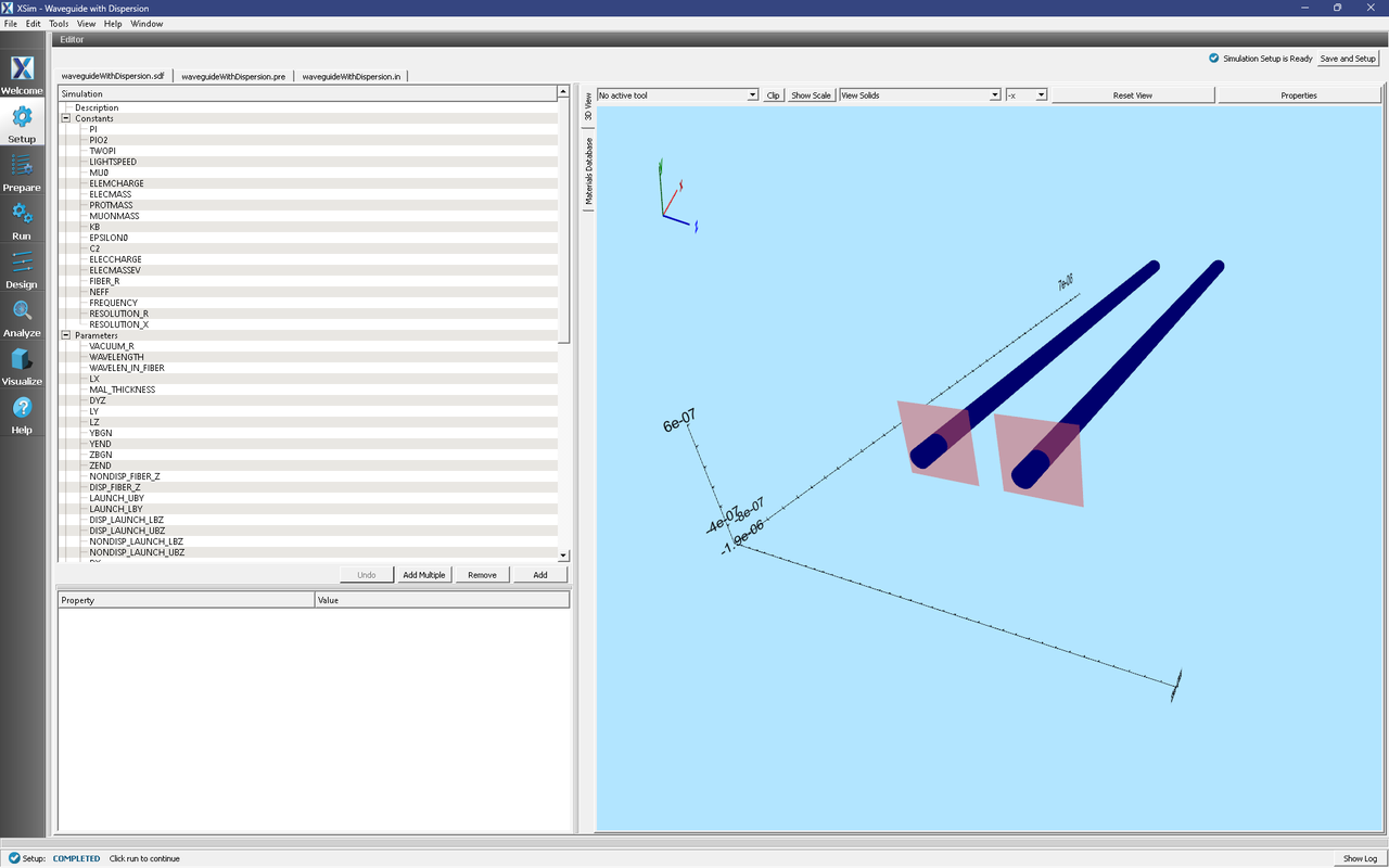
Fig. 287 Initial setup window showing the pair of waveguides and wave launchers.
Simulation Variables
FREQUENCY: Waveguide mode frequency
FIBER_R: Radius of the dielectric cylinders
VACUUM_R: Distance (in y and z) to simulation boundaries from each fiber axis
RESOLUTION_R: Number of grid cells per fiber radius in y and z directions
RESOLUTION_X: Number of grid cells per wavelength (wavelength in fiber)
LAUNCH_X: Location of the waveguide cross-sections; this will be used by the mode solver and the wave launcher
LAUNCH_FREQ_LO: Lower end of the frequency band of the launched pulse (a wider frequency band will give a shorter pulse). Reducing the bandwidth reduces the effects of curvature in the Lorentz dispersion model of \(\varepsilon(\omega)\).
LAUNCH_FREQ_HI: Upper end of the frequency band of the launched pulse.
NEFF: Effective index of refraction of guided mode at FREQUENCY. This can be obtained from the output of the computeWaveguideModes.py analyzer.
MAL_THICKNESS: Thickness of absorbing layers at the lower and upper x boundaries.
There are other variables defined in this simulation, but they are mostly aids to geometry setup. Peruse these if you wish.
Setting up the Preliminary Simulation
The first stage of this example finds waveguide eigenmodes for each fiber. Since the computeWaveguideModes.py analyzer does not yet handle Lorentz materials, we will need to evaluate our 2nd-order dispersive dielectric approximation at our working frequency (FREQUENCY).
In the Setup window, just to the left of the 3D View, click on the Materials Database tab (the tab is oriented vertically). You should then see Fig. 288. In this example, there are three materials, two Lorentz and one regular. Notice how Lorentz materials are specified by sampling a frequency-dependent dielectric function. In this case, we have 2 samples.
The regular dielectric material is in the database only because the computeWaveguideModes.py analyzer will not work with Lorentz materials. This is not a problem, since it is straightforward to create a regular dielectric material that is a sample of a frequency-dependent dielectric function (using a text editor, have a look at the waveguideWithDispersion.vmat file included in this example).
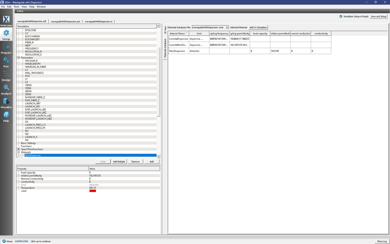
Fig. 288 The custom materials database for this example. It contains a dispersive and non-dispersive Lorentz dielectric material, and a regular non-dispersive dielectric. The regular dielectric matches the non-dispersive Lorentz material, and its dielectric constant is halfway between the samples of the dispersive Lorentz dielectric. Since the dispersion is nearly linear, we have also set our working frequency (FREQUENCY) to be halfway between the sample frequencies in the Lorentz dielectric.
As shown in Fig. 288, the regular non-dispersive dielectric has already been added to the simulation. We will revisit the Materials Database viewer later when we enable the Lorentz dielectric algorithm. As given, the two waveguides shown in 3D View have already been assigned the regular non-dispersive material. Additionally, notice that the waveguide mode launchers under Field Dynamics → CurrentDistributions have been deactivated.
We can now proceed to the Run window and execute the preliminary simulation.
Running the Preliminary Simulation
After performing the above actions, continue as follows:
Proceed to the Run Window by pressing the Run button in the left column of buttons. If you changed something in the setup, you will be asked to Save. Click Save upon the request to save.
In the left pane :
Set Number of Steps to 1
Set Dump Periodicity to 1.
Check Dump at Time Zero.
Click on the Run button in the upper left corner of the right pane.
You will see the output of the run in the right pane. The run has completed when you see the output, “Engine completed successfully”. This result is shown in Fig. 289.
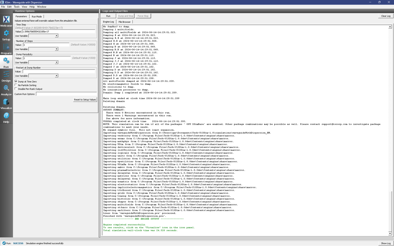
Fig. 289 Running the simulation for one step to get the permittivity data for the analyzer.
Solving for the Eigenmodes
Proceed to the Analyze Window by clicking the Analyze button on the left. There should be two copies of the computeWaveguideModes.py analyzer already open. The first copy is for the non-dispersive fiber, and the second is for the dispersive fiber; one can tell the difference by the variable names used as inputs to each analyzer.
simulationName: waveguideWithDispersion
datasetName: invEps
transverseSliceX: LAUNCH_X
transverseSliceLY: LAUNCH_LBY
transverseSliceUY: LAUNCH_UBY
transverseSliceLZ: NONDISP_LAUNCH_LBZ or DISP_LAUNCH_LBZ
transverseSliceUZ: NONDISP_LAUNCH_UBZ or DISP_LAUNCH_UBZ
vacWavelength: WAVELENGTH
nModes: 1
writeFieldProfile: D
writeFieldNamePrefix: NonDisp or Disp
modeFileName: mode
Normalize: checked
compMajorC: checked
Overwrite: checked
Click Analyze in the top right corner on both copies. The results should resemble Fig. 290. We see that the analyzer found the fundamental mode and gives the effective index of the mode under Neff. This parameter is necessary for using the Waveguide Mode Launcher to launch a unidirectional wave. This value is saved as the constant NEFF in Setup.
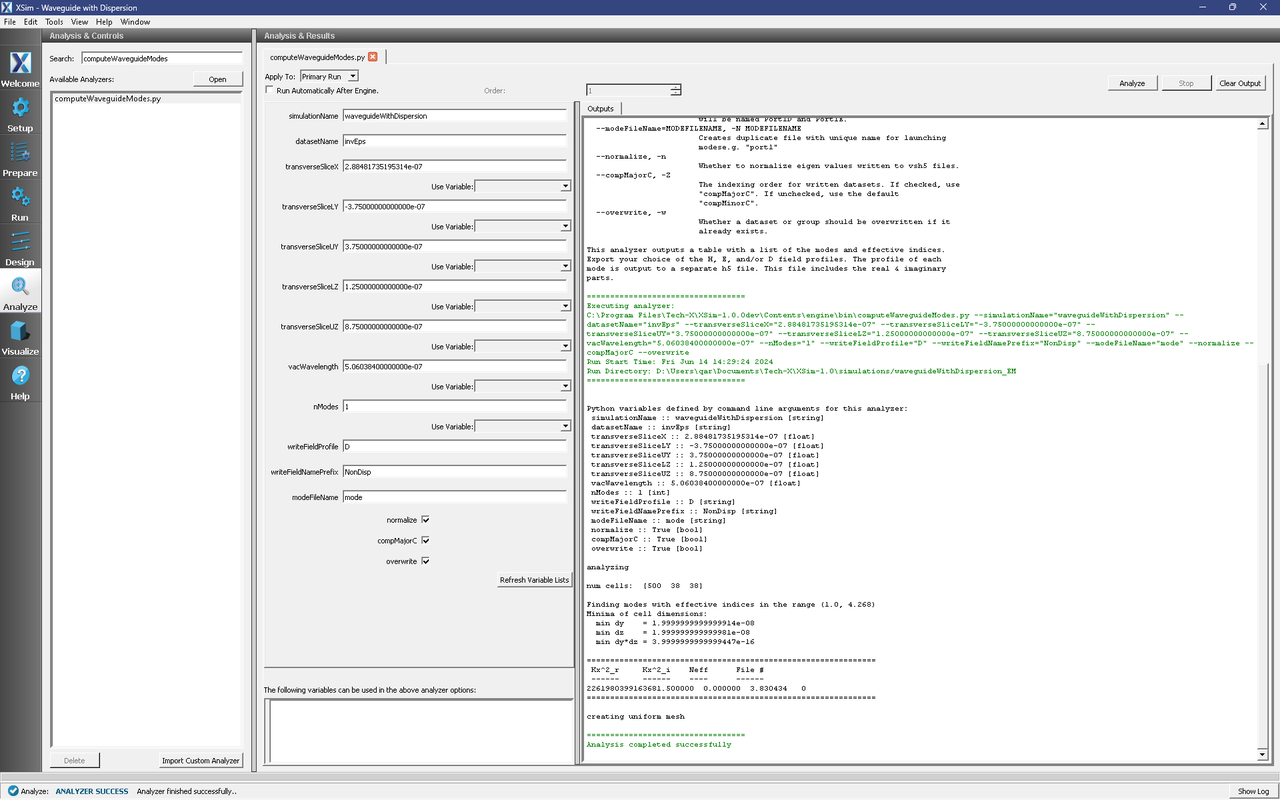
Fig. 290 The analyzer window after a successful run of computeWaveguideModes.py.
If you wish to visualize the waveguide modes, proceed to the Visualize window by clicking the Visualize tab on the left. To see the mode patterns overlaid on the waveguides at the launch points, go to the Variables tree, and expand and select the following:
Scalar Data → DispD → DispD_magnitude
Scalar Data → NonDispD → NonDispD_magnitude
Geometries → dispFiberBoundaryTriangles
Geometries → nonDispFiberBoundaryTriangles
You should see Fig. 291.

Fig. 291 Visualizing the modes from computeWaveguideModes.py and the waveguide geometries.
Setting up the Main Simulation
Return to the Setup window by pressing the Setup button on the left. Recall that, to find the waveguide modes, we sampled the dispersive dielectric function at a single frequency using a standard dielectric material. We now wish to simulate the dispersive dielectric using the Lorentz-model algorithm and watch pulses propagate at different group velocities in each fiber.
The Lorentz model algorithm applies to the entire simulation; therefore, we need to assign all objects a “dispersive” material, even if the dielectric function is flat. There are several steps to this process.
First, we need to disassociate the regular dielectric material from the fiber geometries. In the Simulation tree, expand Geometries → CSG and select nonDispFiberBoundary. In the Property pane below, double-click on the material property (it should be set to the NonDispersive material), and select the blank entry from the dropdown. Repeat this for Geometries → CSG → dispFiberBoundary.
Next, expand Materials, select the the NonDispersive material, and then click the Remove button below. There should be no remaining materials in the Simulation tree.
We now add the dispersive dielectric materials to the simulation. Return to the Materials Database viewer by clicking on the vertically-oriented Materials Database tab. In the database, select the material named LorentzDispersive, then click the Add To Simulation button above the database pane. Repeat this for the material with name LorentzNonDispersive. You should see both of these materials in the Simulation tree to the left. See Fig. 292 for reference.
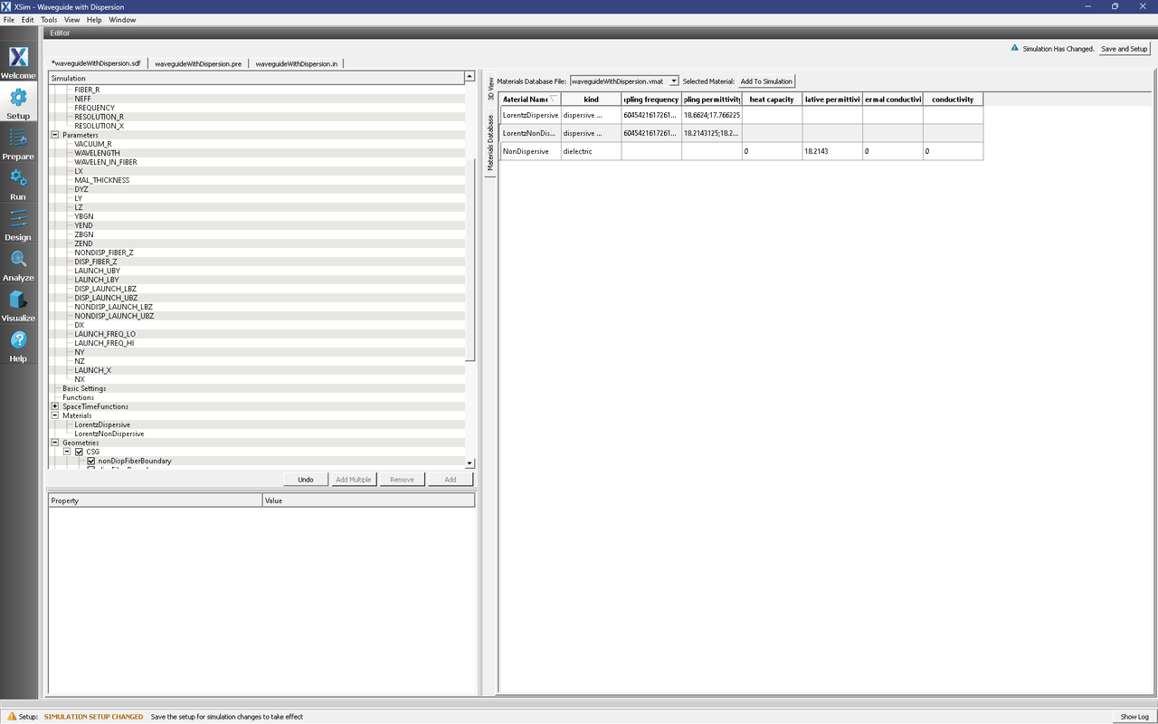
Fig. 292 The result of removing the NonDispersive regular dielectric material from the simulation, and adding the Lorentz materials.
Next, select Basic Settings in the Simulation tree, and find field solver → Lorentz resonances in the pane below. It should currently say none. Double click none and replace it with the following frequency: 810249886486486.5. (see Fig. 293 for reference). This resonant frequency is far above our working frequency, and thus the dispersion will be weak (and nearly linear) for our waveguide mode pulse.
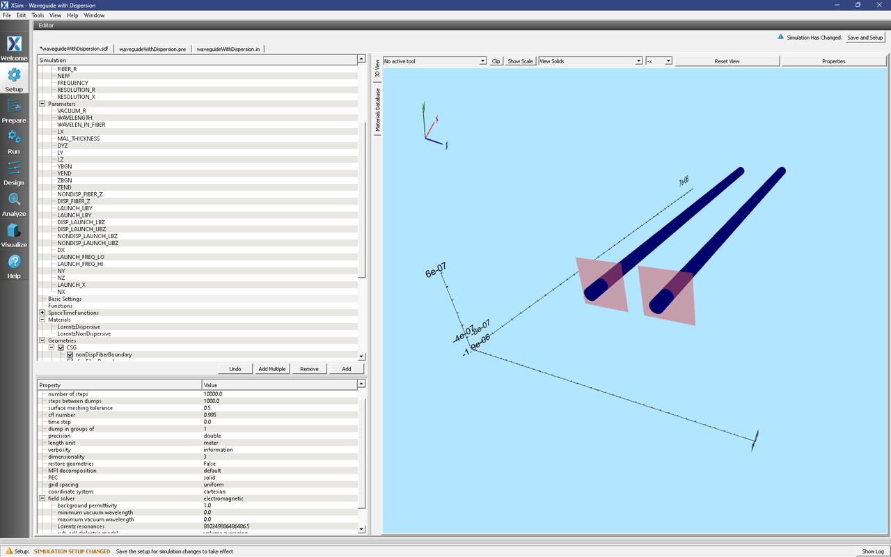
Fig. 293 Setting the Lorentz resonant frequency in Basic Settings.
Revisit the fiber geometries in the Simulation tree at Geometries → CSG. Select nonDispFiberBoundary and, in the pane below, assign the LorentzNonDispersive material to the geometry. Next, select dispFiberBoundary and assign the LorentzDispersive material to this geometry. See Fig. 294.
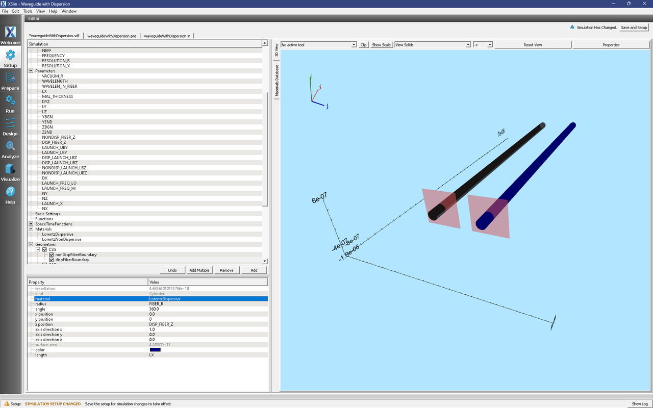
Fig. 294 Assigning Lorentz material to a fiber geometry.
Finally, activate the waveguide mode launchers:
Expand Field Dynamics
Expand CurrentDistributions
Right Click on nonDispWaveguideModeLauncher
Left click on Activate
Right Click on dispWaveguideModeLauncher
Left click on Activate
Click on Save and setup in the top right corner. Activation of the waveguide mode launcher should look like Fig. 295.
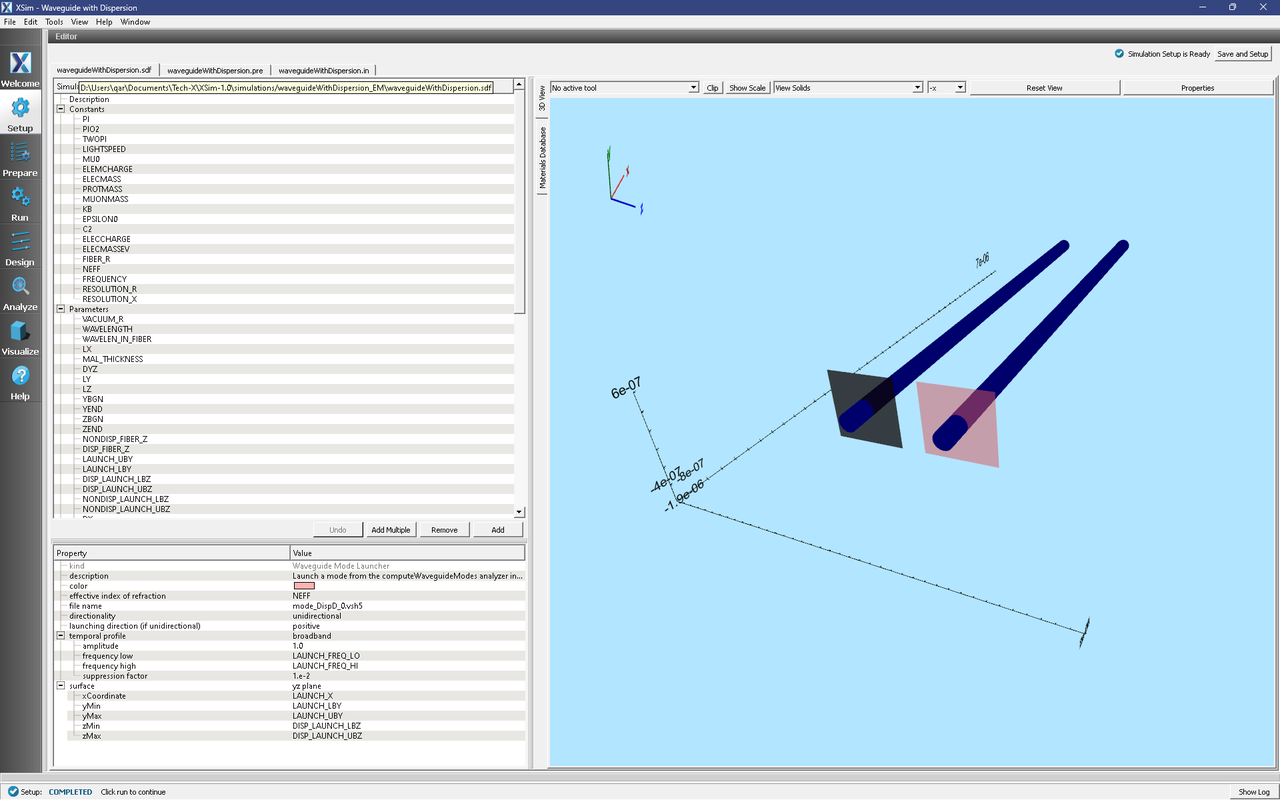
Fig. 295 Activating the waveguide mode launchers.
Running the Main Simulation
After performing the above actions, continue as follows:
Proceed to the Run Window by pressing the Run button in the left column of buttons. You will be asked to Save. Click Save upon the request to save.
In the left pane, click on Reset to Setup Values to run for enough steps to see the modes propagate.
Check Dump at Time Zero.
Click on the Run button in the upper left corner of the right pane.
You will see the output of the run in the right pane. The run has completed when you see the output, “Engine completed successfully.” This result is shown in Fig. 296.
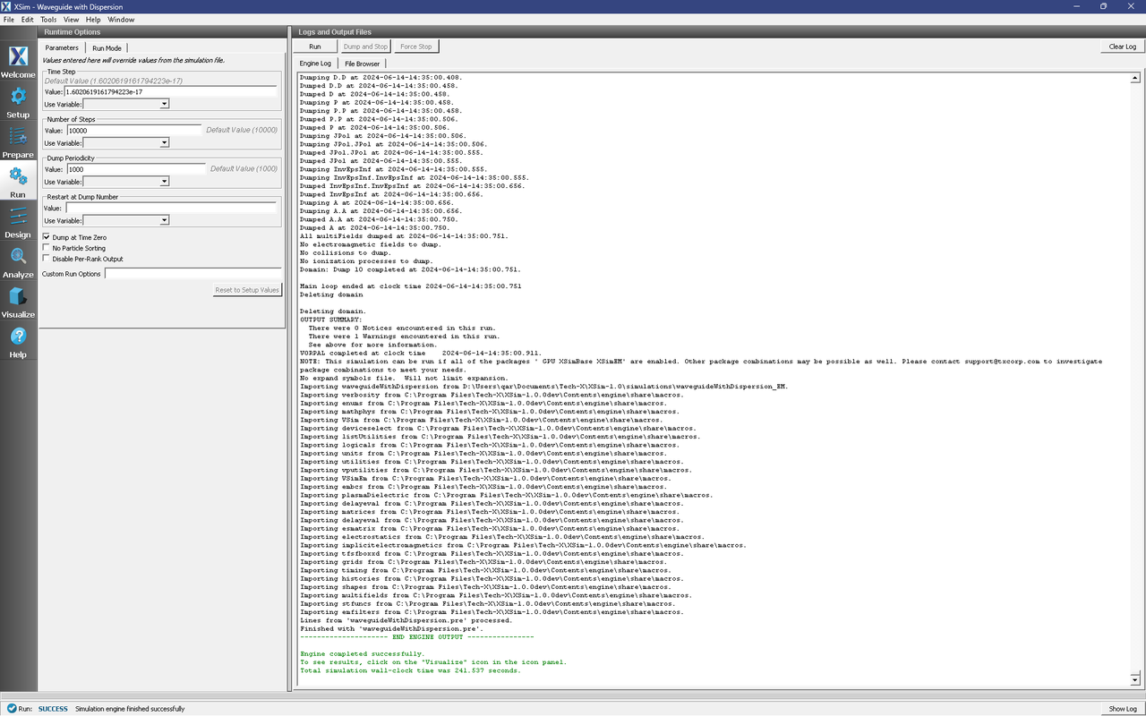
Fig. 296 Running the full simulation which launches this wave down the waveguide.
Visualizing the Results
Proceed to the Visualize Window by pressing the Visualize button in the left column of buttons. You may need to Reload Data (top right). If the eigenmodes (DispD and NonDispD) are still displayed over the fiber geometries, uncheck all checked items in the Variables tree.
Expand Scalar Data → D and check D_magnitude. In the pane below, check Clip plot and then click the Plane Controls button. In the resulting dialog, uncheck Plane3, check Plane2, and click Ok. Below the 3D view, slide to Dump: 7 and rotate the 3D view until you can see the pulses in the waveguides. You should see something like Fig. 297.
Notice that one of the pulses is weaker in magnitude and slower. This is the pulse in the fiber with dispersive dielectric. We expect the pulse to be slower because the dielectric constant increases with frequency. We are also not surprised that the launched mode is more weakly-coupled to the waveguide; this may be due to the finite-difference approximation of the Lorentz model or the fact that the Lorentz model is not perfectly linear (but close) between our samples of the dielectric function.
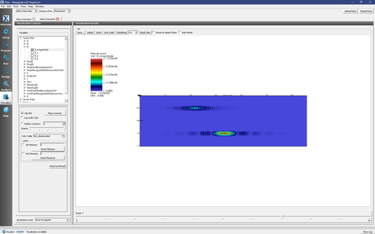
Fig. 297 Visualizing the propagating pulses. The slower pulse is in the fiber with the dispersive dielectric.