Three Material Waveguide (threeMaterialWaveguide.sdf)
Keywords:
- Photonic Waveguide, Guided Mode, Semiconductor
Problem Description
This example demonstrates how to calculate and launch the fundamental mode of a rectangular silicon waveguide using a unidirectional waveguide mode launcher and a broadband signal. In this example, the waveguide itself is sitting on top of a silica slab and is surrounded on the other 3 walls by quartz.
This simulation can be performed with a XSimEM license.
Opening the Simulation
To open this example open an instance of XSimComposer and follow the steps below:
Select the New → From Example… menu item in the File menu.
In the resulting Examples window expand the XSim for Electromagnetics option.
Expand the Photonics option.
Select Three Material Waveguide and press the Choose button.
In the resulting dialog, create a New Folder if desired, and press the Save button to create a copy of this example.
Simulation Variables
This example contains a number of variables defined to make the simulation easily modifiable.
CPWX and CPWYZ: CPWX controls the number of cells per vacuum wavelength in the x direction and CPWYZ controls the number of cells per vacuum wavelength in both the y and z directions. Increasing one or both of these values will increase the resolution of the simulation.
WAVELENGTH: Center wavelength of the input signal. This wavelength is also used for the calculation of the fundamental guided mode of the device.
WAVEGUIDE_WIDTH and WAVEGUIDE_HEIGHT: These two parameters control the cross sectional area of the waveguide.
The Materials section contains silicon, silica, and quartz. The Geometries section includes the CSG waveguide, the silica slab, and their defining parameters. In this example, filling the rest of the empty space with quartz is done by going to the Basic Settings section and setting the background permittivity variable to 4.5. In Field Dynamics, there are FieldBoundaryConditions and CurrentDistributions to be aware of. In photonics simulations, Matched Absorbing Layers (MALs) are the most stable boundary conditions for preventing reflections. This simulation makes use of XSim’s Waveguide Mode Launcher to launch a unidirectional wave down the waveguide with a mode defined by the file generated by the computeWaveguideModes.py analyzer.
Solving for the Eigenmodes
To calculate the fundamental mode of the silicon waveguide, first make sure that in the Setup tab that waveguideModeLauncher0 is set to inactive. Save the simulation and proceed to the Run tab. Set Number of Steps and Dump Periodocity to 1 and make sure that Dump at Time Zero is checked. Click on the Run button. Upon successful completion of the engine, proceed as follows:
Proceed to the Analyze Window by clicking the Analyze button on the left.
Select computeWaveguideModes.py and click Open under the list.
Update the analyzer fields accordingly by choosing the corresponding variables under Use Variable :
simulationName: threeMaterialWaveguide
datasetName: invEps
transverseSliceX: PORT_BGNX
transverseSliceLY: PORT_BGNYZ
transverseSliceUY: PORT_ENDYZ
transverseSliceLZ: PORT_BGNYZ
transverseSliceUZ: PORT_ENDYZ
vacWavelength: 1.55e-6
nModes: 1
writeFieldProfile: D
writeFieldNamePrefix: Eigen
modeFileName: port1
Normalize: checked
compMajorC: checked
Overwrite: checked
Click Analyze in the top right corner.
The analyzer will only find guided modes. The results should resemble Fig. 270. We see that the analyzer found the fundamental mode and gives the effective index of the mode under Neff. This parameter is necessary for using the Waveguide Mode Launcher to launch a unidirectional wave. This value is saved as a parameter as NEFF.
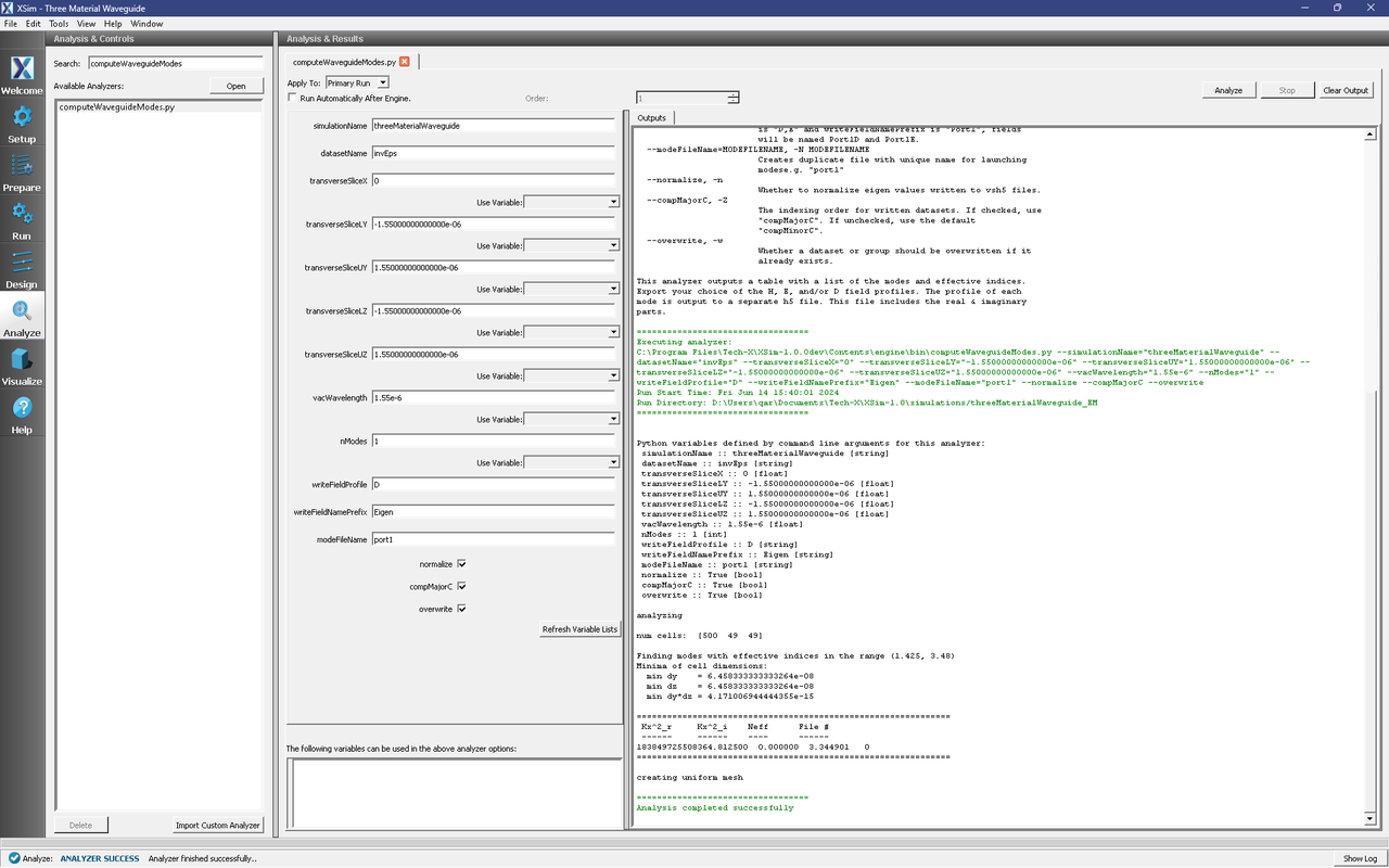
Fig. 270 The analyzer window after a successful run of computeWaveguideModes.py.
Setting up the Simulation
After performing the above actions, continue as follows:
Proceed to the Setup Window by pressing the Setup button in the left column of buttons.
Activate the waveguide mode launcher
Expand Field Dynamics
Expand CurrentDistributions
Right Click on waveguideModeLauncher0
Left click on Activate
Click on Save and setup in the top right corner.
This setting is shown in Fig. 271.
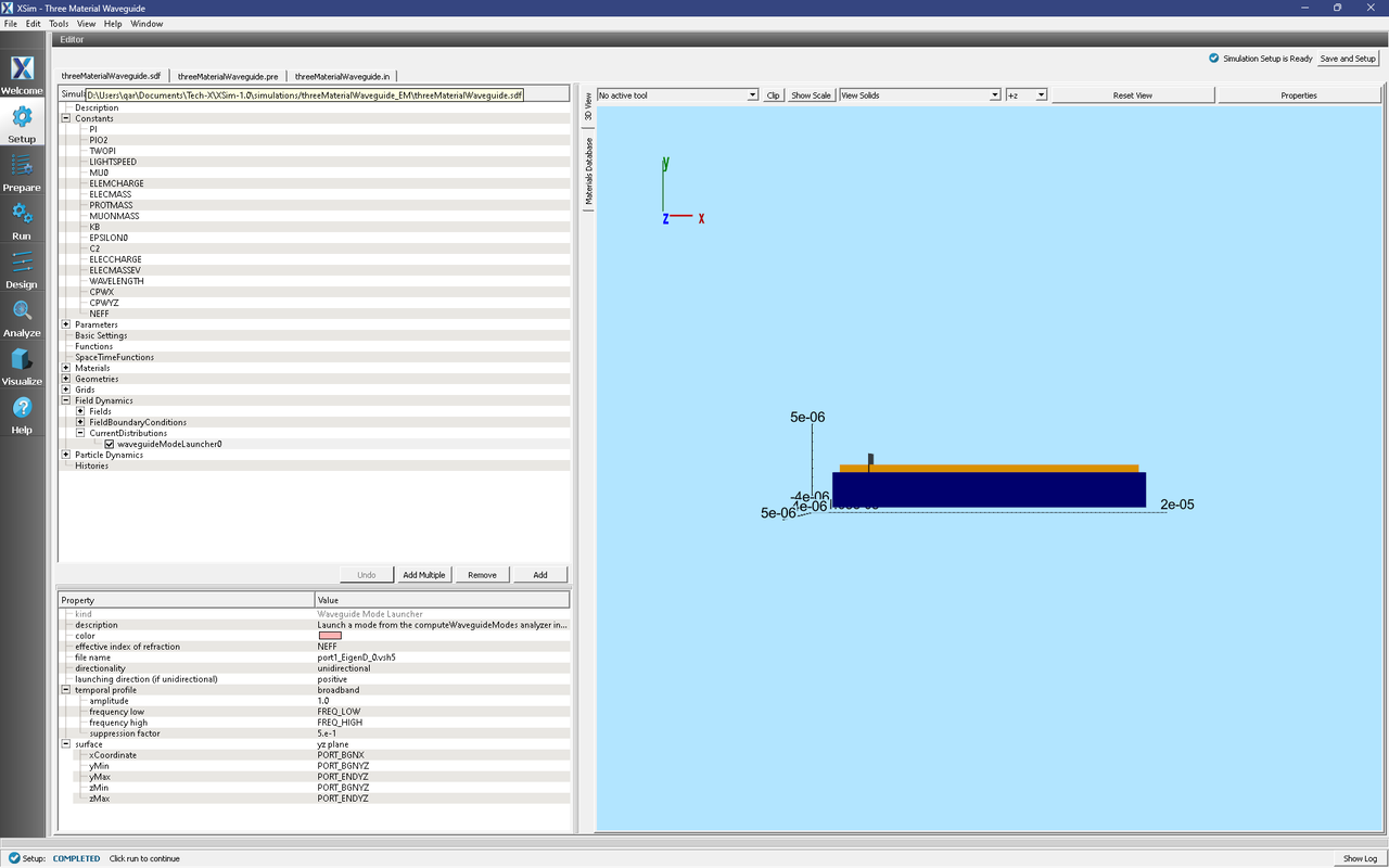
Fig. 271 Location of waveguideModeLauncher0 within the setup tree.
Running the Simulation
After performing the above actions, continue as follows:
Proceed to the Run Window by pressing the Run button in the left column of buttons. You will be asked to Save. Click Save upon the request to save.
In the left pane, click on Reset to Setup Values to run the full simulation which launches this wave down the waveguide.
Check Dump at Time Zero.
Click on the Run button in the upper left corner of the right pane.
Click Delete and Run when prompted.
You will see the output of the run in the right pane. The run has completed when you see the output, “Engine completed successfully.” This result is shown in Fig. 272.
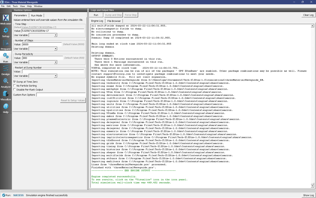
Fig. 272 Running the full simulation which launches the wave down the waveguide.
Visualizing the Results
After performing the above actions, continue as follows:
Proceed to the Visualize Window by pressing the Visualize button in the left column of buttons.
You may need to Reload Data (bottom left). Visualize an eigenmode by following these steps:
From the Add a Data View dropdown, select Data Overview.
Expand Scalar Data, expand EigenD, and select EigenD_magnitude.
In the Visualization Results window, change the viewing direction from +z (the default) to -x to see the mode.
Optionally expand Geometries and select wavguideTriangles to see both the mode and the tesselation of the waveguide.
The resulting visualization pane should look like Fig. 273. The offset of the mode pattern from the geometry is merely an artifact of the rendering—the pattern is actually centered when considering the half-cell offset of field components on the Yee finite-difference grid.
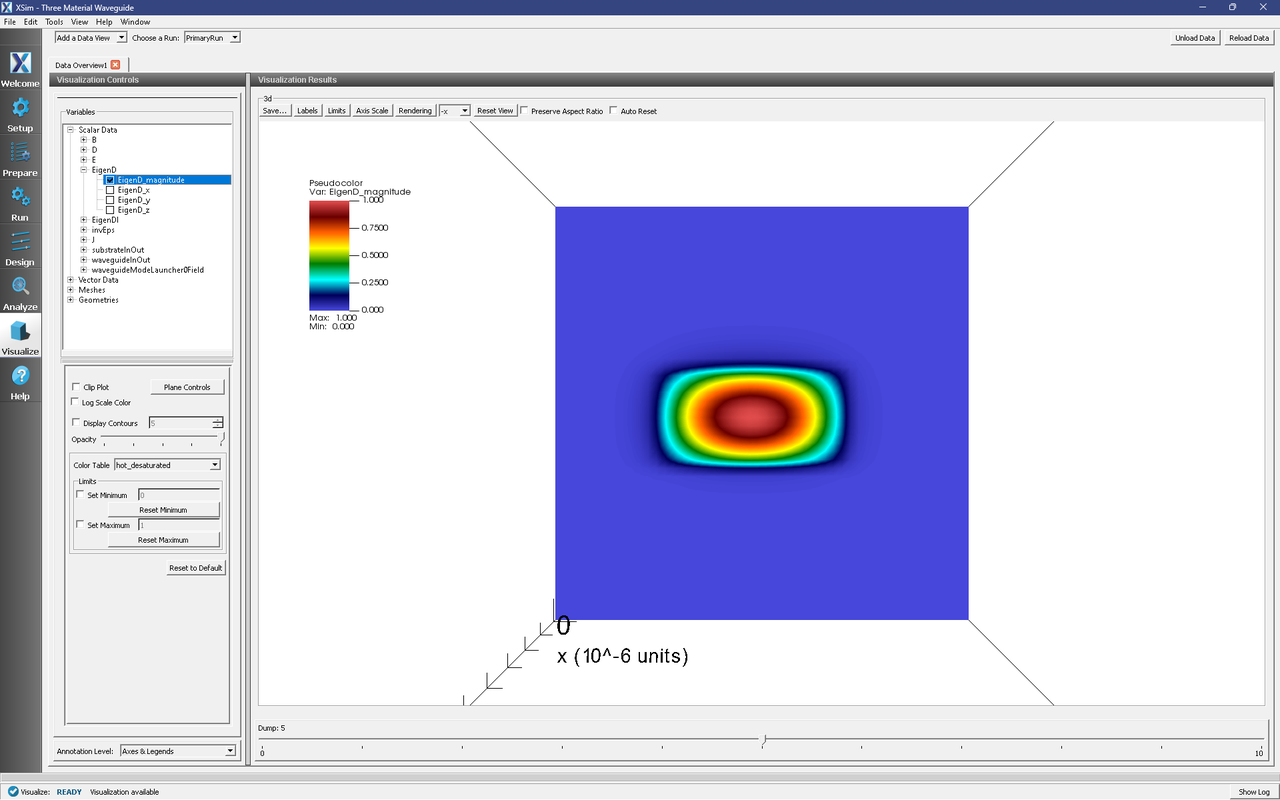
Fig. 273 The visualization pane showing the magnitude of the D field of the fundamental mode with the waveguide geometry overlaid.
To visualize the E field as it travels down the waveguide, proceed as follows:
From Data Overview, expand Scalar Data, expand E, then select E_z.
Slide the dump number selector over to the right to watch the wave travel down the waveguide.
The resulting visualization pane should look like Fig. 274.
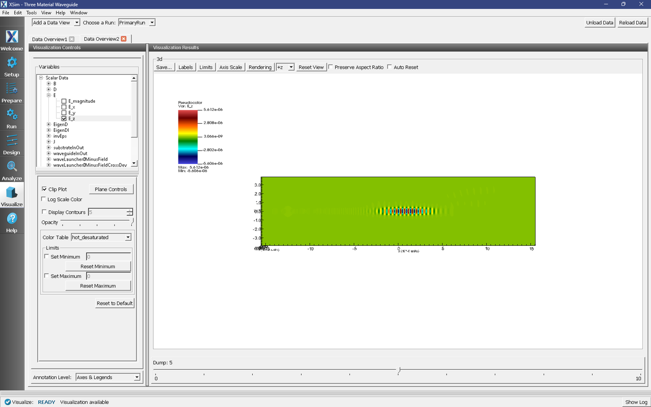
Fig. 274 The visualization pane showing the z component of the E field.
If instead you wish to view a cross section of the waveguide and E field, proceed as follows:
From Data Overview, expand Scalar Data, expand E, then select E_z.
In the visualization controls section, click on the Plane Controls button. Deselect Plane3 and select Plane1. Click the Apply button. Click Ok.
In the visualization results view, to the left of the Reset View button is a drop down menu. Change this to +x.
To make the field outside of the waveguide, change the minimum and maximum values under Limits to -5e-6 and 5e-6.
The resulting visualization pane should look like Fig. 275.
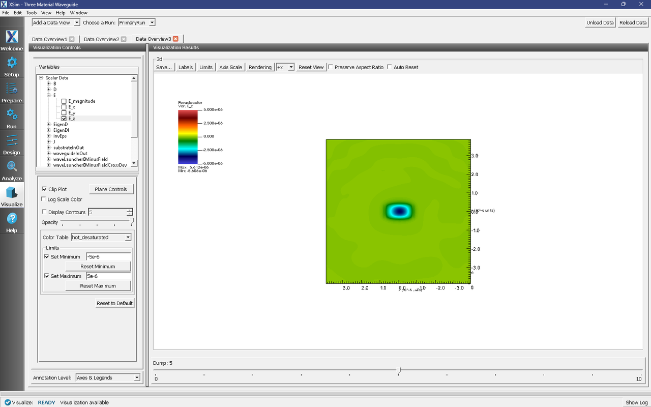
Fig. 275 The visualization pane showing the z component of the E field in a cross section of the domain.
Further Experiments
Change the geometry on the Setup window and rerun the simulation and analyzer to see the effects on the modes. Change the materials used and see how the field inside and outside the waveguide changes.