Cylindrical Dielectric Waveguide Mode with Variable Grid (cylinderWaveguideDielectricVarGrid.sdf)

Keywords:

Photonic Waveguide, Waveguide Mode Solver, Guided Mode, Variable Grid

Problem Description

This example demonstrates finding and launching a guided mode into a dielectric waveguide. The waveguide is a simple dielectric cylinder, but the process is the same for more complicated waveguide cross sections that may be a small part of a more complex simulation. This example also uses a variable grid, showcasing the generality of the waveguide mode solver. Since guided modes have their energy concentrated in the waveguide, we can reduce computation (without sacrificing accuracy) by using a variable grid to resolve the waveguide better than the surrounding vacuum.

The cylinder waveguide in our simulation has its axis in the x direction, and so eigenmodes take the form:

\[\mathbf{E}(\mathbf{x},t) = \mathbf{E}(y,z) e^{i(k x - \omega t)}\]

The effective index of refraction of a waveguide mode is given by \(\bar{n} = k / k_0\) where \(k_0 = \omega / c\). If the waveguide has index of refraction \(n_w\) and the cladding \(n_c < n_w\), then a guided mode will have a modal index in the range, \(n_c < \bar{n} < n_w\) (in our case, \(n_c=1\)).

The high-level overview of the waveguide solve-and-launch process is roughly:

• Set up the simulation (geometries, materials, grid, etc.)

• Run for 1 time step to generate finite difference matrices

• Run the computeWaveguideModes.py analyzer on a cross-section of the waveguide

• Identify the desired mode and its number in the Visualize tab

• Set up and run the mode launcher with the desired mode

This simulation can be performed with a XSimEM license.

Opening the Simulation

To open this example open an instance of XSimComposer and follow the steps below:

• Select the New → From Example… menu item in the File menu.

• In the resulting Examples window expand the XSim for Electromagnetics option.

• Expand the Photonics option.

• Select Cylindrical Dielectric Waveguide Mode with Variable Grid and press the Choose button.

• In the resulting dialog, create a New Folder if desired, and press the Save button to create a copy of this example.

As provided, the simulation is set up for the waveguide mode solver process (i.e. the mode launcher is turned off). Before running any tasks, we briefly discuss the simulation setup.

Simulation Variables

This example tries to stay simple while highlighting a few major features: variable grids and the waveguide solver. The following is a partial list of the simulation variables:

• RADIUS: Radius of the dielectric cylinder

• LENGTH: Length of the cylinder

• WAVELENGTH: Vacuum wavelength of the mode to excite

• FREQ: (LIGHTSPEED/WAVELENGTH) Mode frequency

• BANDWIDTH: Frequency bandwidth of launched waveguide mode pulse; inversely proportional to the pulse duration

• CELLS_PER_WAVELENGTH: Resolution in the x direction

• DYZ_FRAC: Transverse size of a grid cell in the cylinder expressed as a fraction of the transverse cell size at the edges of the simulation (DYZ_FRAC < 1); as DYZ_FRAC goes to 0, the cylinder is resolved much better than the simulation edges

• NYZ: Number of cells across the y and z dimensions; this parameter changes the transverse resolution without changing the transverse variation of cell sizes

• LB: Lower bound of the simulation in the y and z directions

• UB: Upper bound of the simulation in the y and z directions

• LAUNCH_X: Location of the waveguide cross-section; this will be used by the mode solver and the wave launcher

• LB_LAUNCH: Lower bound of waveguide cross-section

• UB_LAUNCH: Upper bound of waveguide cross-section

Variable Grid

In this simulation, the cell size varies in the y and z directions only (perpendicular to the cylinder axis). To specify the variation, we fix the number of cells in the y and z directions and set the cell-size ratio using DYZ_FRAC. The cell size decreases linearly from the edges of the simulation to the edge of the waveguide.

As given, this example already has the variable grid set up. The steps to do so were:

• Right click on Grid and select “Create Refinement Region”

• Set the refinement region parameters as shown in Fig. 276. Notice that the cell sizes specified here are relative to the cell sizes at the simulation edges (see next step).

• Click on Grid and change the boundary cell size behavior to manualCellSizing, and set all cell sizes at the simulation edges to 1 (see Fig. 277)

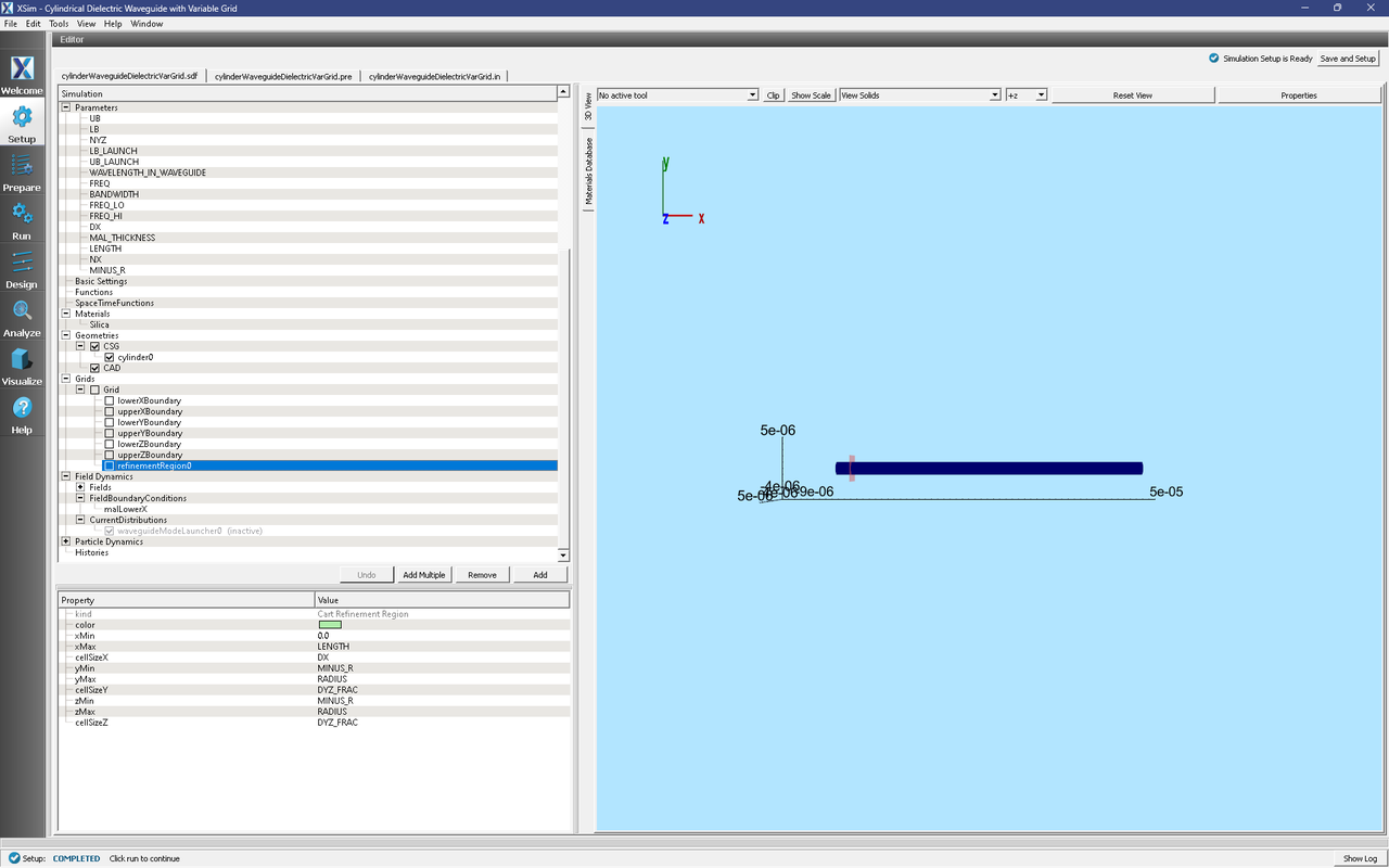
Fig. 276 Grid refinement parameters. Cell sizes grow linearly from the waveguide edge to the simulation edge.

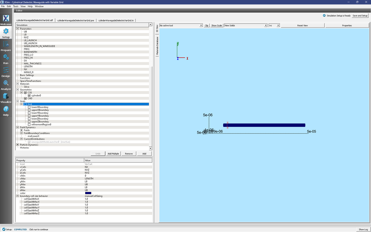
Fig. 277 The cell size at the simulation boundaries was set to 1 so that the cell size in the waveguide could be set with a relative value, DYZ_FRAC < 1.

Setting up the Preliminary Simulation

As delivered, the system is set up to generate the data needed to run the computeWaveguideModes.py analyzer. To ensure that your simulation has second order accuracy, under Basic Settings, verify that the dielectric solver field is set to volume averaging. It is also necessary to make sure the wave launcher is deactivated before running the first simulation since the waveguide mode file is not generated until the computeWaveguideModes.py analyzer is run. To deactivate, expand Field Dynamics, expand CurrentDistributions and verify that waveguideModeLauncher0 is {inactive}.

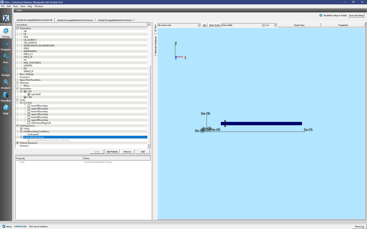
Fig. 278 The inactive waveguide mode launcher.

Running the Preliminary Simulation

After performing the above actions, continue as follows:

• Proceed to the Run Window by pressing the Run button in the left column of buttons. If you changed something in the setup, you will be asked to Save. Click Save upon the request to save.

• In the left pane :

  • Set Number of Steps to 1

  • Set Dump Periodicity to 1.

  • Check Dump at Time Zero.

• Click on the Run button in the upper left corner of the right pane.

You will see the output of the run in the right pane. The run has completed when you see the output, “Engine completed successfully”. This result is shown in Fig. 279.

Fig. 279 Running the simulation for one step to get the permittivity data for the analyzer.

Solving for the Eigenmodes

As provided, the computeWaveguideModes.py analyzer should already be open in the Analyze tab. The steps to set it up were as follows:

• Proceed to the Analyze Window by clicking the Analyze button on the left.

• Select computeWaveguideModes.py and click Open under the list.

• Update the analyzer fields to

  • simulationName: cylinderWaveguideDielectricVarGrid

  • datasetName: invEps

  • transverseSliceX: MAL_THICKNESS

  • transverseSliceLY: LB_LAUNCH

  • transverseSliceUY: UB_LAUNCH

  • transverseSliceLZ: LB_LAUNCH

  • transverseSliceUZ: UB_LAUNCH

  • vacWavelength: WAVELENGTH

  • nModes: 1

  • writeFieldProfile: D

  • writeFieldNamePrefix: Eigen

  • modeFileName: port1

  • Normalize: checked

  • compMajorC: checked

  • Overwrite: checked

• Click Analyze in the top right corner.

The analyzer will only find guided modes. The results should resemble Fig. 280. We see that the analyzer found the fundamental mode and gives the effective index of the mode under Neff. This parameter is necessary for using the Waveguide Mode Launcher to launch a unidirectional wave. This value should be entered as the constant NEFF in the Setup window.

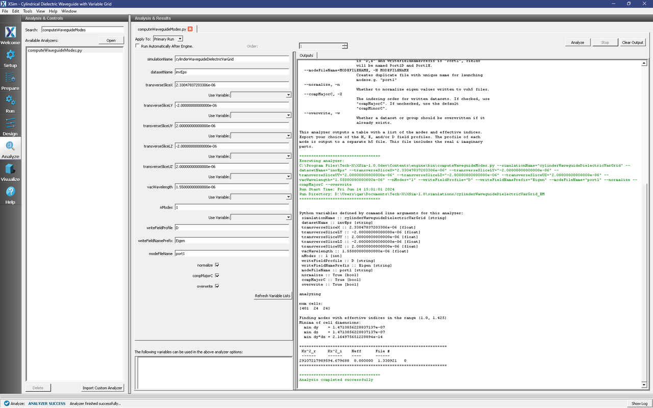
Fig. 280 The analyzer window after a successful run of computeWaveguideModes.py.

Setting up the Main Simulation

After performing the above actions, continue as follows:

• Proceed to the Setup Window by pressing the Setup button in the left column of buttons.

• Expand Constants and make sure NEFF matches the value printed by the computeWaveguideModes.py analyzer.

• Activate the wave launcher:

  • Expand Field Dynamics

  • Expand CurrentDistributions

  • Right Click on waveguideModeLauncher0

  • Left click on Activate

• Click on Save and setup in the top right corner.

The active waveguide mode launcher is shown in Fig. 281.

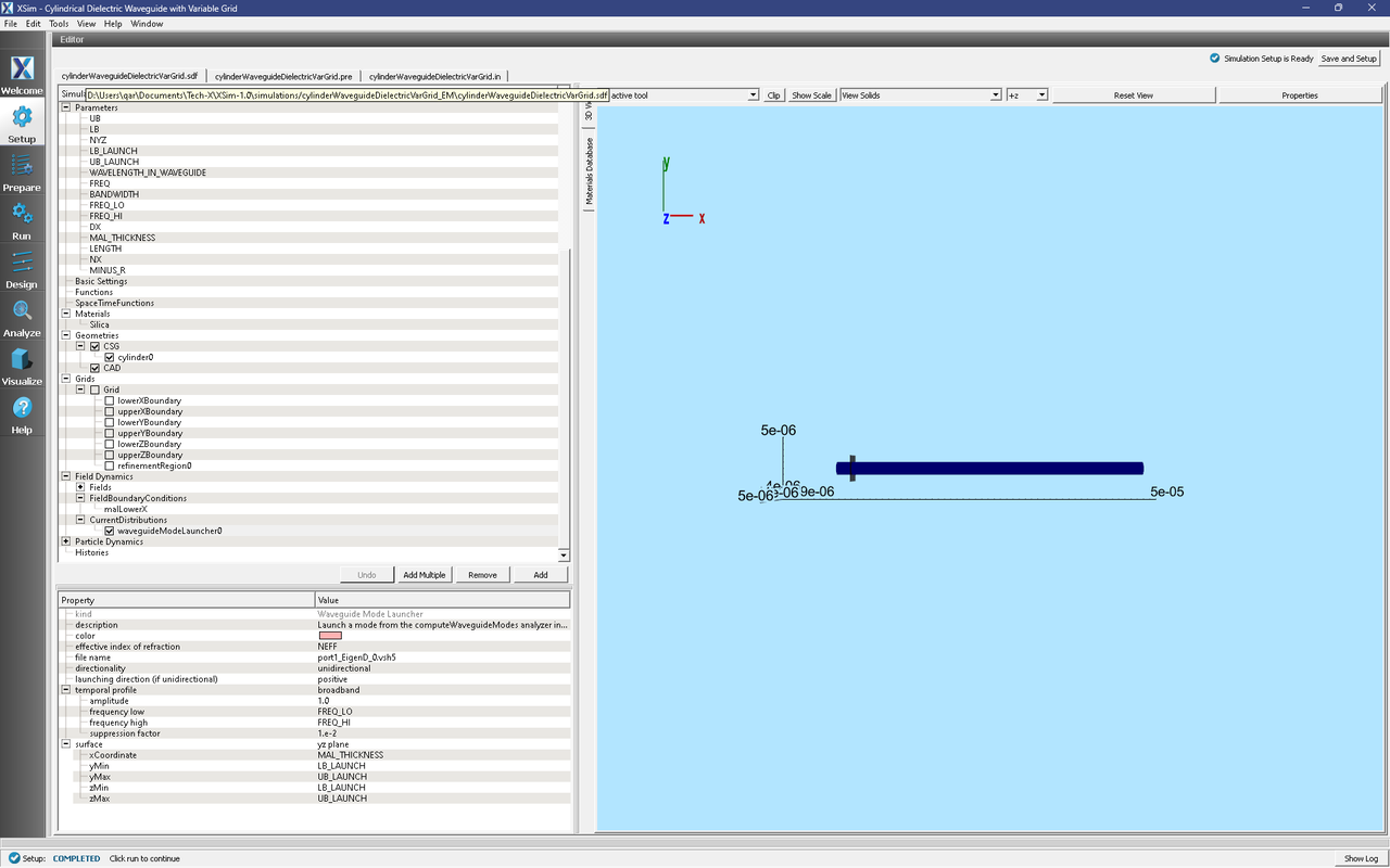
Fig. 281 Activating the waveguide mode launcher.

Running the Main Simulation

After performing the above actions, continue as follows:

• Proceed to the Run Window by pressing the Run button in the left column of buttons. You will be asked to Save. Click Save upon the request to save.

• In the left pane, click on Reset to Setup Values to run the full simulation which launches this wave down the waveguide.

• Check Dump at Time Zero.

• Click on the Run button in the upper left corner of the right pane.

You will see the output of the run in the right pane. The run has completed when you see the output, “Engine completed successfully.” This result is shown in Fig. 282.

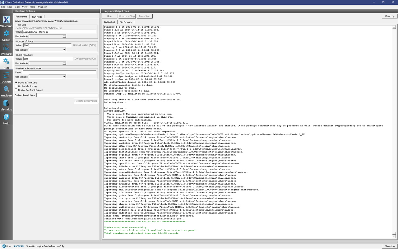
Fig. 282 Running the full simulation which launches this wave down the waveguide.

Visualizing the Results

After performing the above actions, continue as follows:

• Proceed to the Visualize Window by pressing the Visualize button in the left column of buttons.

You may need to Reload Data (top right). Visualize an eigenmode by following these steps:

• From the Add a Data View dropdown, select Data Overview.

• Expand Scalar Data, expand EigenD, and select EigenD_magnitude.

• Additionally expand Geometries and select cylinder0Triangles to see the mode pattern overlaid on the waveguide geometry at the launch point.

The resulting visualization pane should look like Fig. 283.

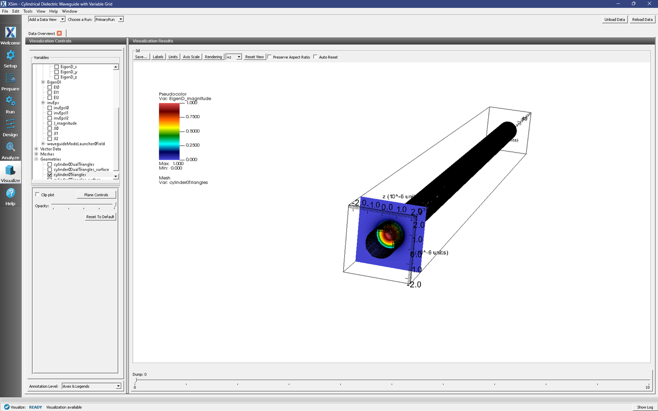
Fig. 283 The visualization pane showing the magnitude of the D field of the fundamental mode.

We can also visualize the launched waveguide mode by changing our Scalar Data selection to only D_magnitude and checking the Clip Plot option that appears below the Variables tree. After moving the dump slider to Dump: 6, we should see a pulse that looks like Fig. 284.

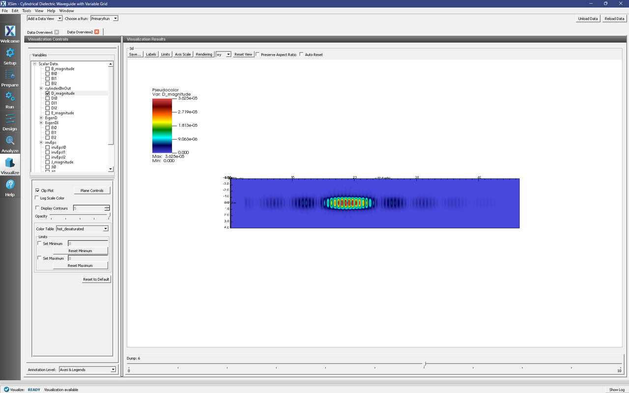
Fig. 284 The visualization pane showing the magnitude of a waveguide mode pulse propagating down the waveguide.

Further Experiments

Change the geometry on the Setup window and rerun the simulation and analyzer to see the effects on the modes. Once you have your desired mode, launch it down the waveguide using the procedures laid out above.

One can run a full convergence study of the waveguide eigenmode by repeating the following process as many times as desired:

• Deactivate the waveguide mode launcher (should only need to do this once).

• Change the transverse resolution (NYZ) in the Setup window.

• Run for 1 time step.

• Run the computeWaveguideModes.py analyzer and record the wavenumber (Kx) or effective index (Neff).

The above can also be automated. In the XSim Design window, select variable NYZ from the Add Parameter dropdown. Choose a range of values for NYZ by setting the options that appear below the parameter list:

• Model Choice: Range

• Number of Points: any (10 points with Min=20 and Max=200 will increment by 20)

• Min: 20

• Max: 200 (included in range)

The Run Status window should show something like Fig. 285.

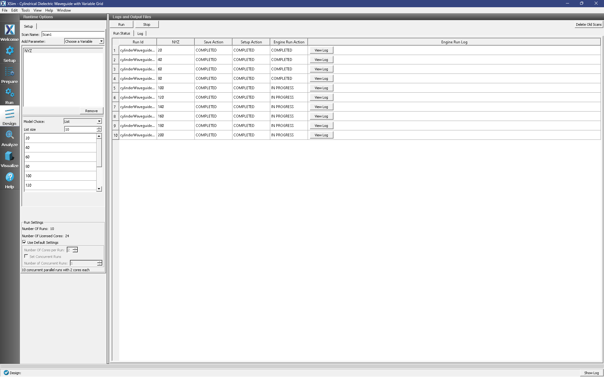
Fig. 285 The Design window showing a parameter scan over 10 equally-spaced values of NYZ.

The computeWaveguideModes.py analyzer can be applied to all the runs of the parameter scan by going to the Analyze window, and selecting All Runs from the Apply To: dropdown. After copying and pasting the analyzer output (from all runs) to a text file, we can write a script to parse and plot the Kx values vs. the transverse grid cell area. Figure Fig. 286 shows such a plot and highlights the second order accuracy of our cut-cell dielectric algorithms.

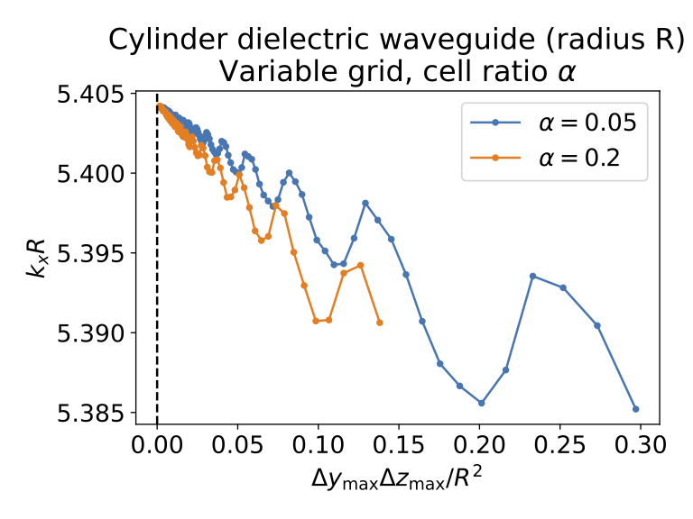
Fig. 286 The wavenumber as a function of transverse cell area for an eigenmode, where \(\alpha\) is DYZ_FRAC.