Dielectric Waveguide Mode Calculation (dielectricWaveguideModeCalc.sdf)
Keywords:
- Mode Extraction, Photonic Waveguide, Guided Mode, Semiconductor
Problem Description
This example demonstrates the process for extracting the effective index and fields of a guided mode by directly solving an eigenvalue equation. The use of permittivity averaging enables second order accuracy in our solution. The waveguide axis runs parallel to the x-axis, and is surrounded by a background cladding with a lower permittivity. We will run the simulation for 1 step and then use the dielectricWaveguideModeCalc_invEps_0.h5 file to solve for the guided modes using the computeWaveguideModes.py analyzer. This analyzer will find the fundamental mode of this waveguide and output this mode into a separate .vsh5 file. This mode file is then used to launch the extracted mode into the simulation using the Waveguide Mode Launcher.
Eigenmodes in such a simulation have the form:
The effective index of refraction of a waveguide mode is given by \(\bar{n} = k / k_0\) where \(k_0 = \omega / c\). If the waveguide has index of refraction \(n_w\) and the cladding \(n_c < n_w\), then a guided mode will have a modal index in the range, \(n_c < \bar{n} < n_w\).
This simulation can be performed with a XSimEM license.
Opening the Simulation
To open this example open an instance of XSimComposer and follow the steps below:
Select the New → From Example… menu item in the File menu.
In the resulting Examples window expand the XSim for Electromagnetics option.
Expand the Photonics option.
Select Dielectric Waveguide Mode Calculation and press the Choose button.
In the resulting dialog, create a New Folder if desired, and press the Save button to create a copy of this example.
Simulation Variables
This example contains a number of variables defined to make the simulation easily modifiable. Notably,
WAVELENGTH_CENTER: Wavelength of the mode in the waveguide.
GEO_CORE_WIDTH: Width of the waveguide.
GEO_CORE_HEIGHT: Height of the waveguide.
The Materials section contains just silicon and silica. The Geometries section includes the CSG waveguide and its defining parameters. In Field Dynamics, there are FieldBoundaryConditions and CurrentDistributions to be aware of. In photonics simulations, Matched Absorbing Layers (MALs) are the most stable boundary conditions for preventing reflections. This simulation makes use of XSim’s Waveguide Mode Launcher to launch a unidirectional wave down the waveguide with a mode defined by the file generated by the computeWaveguideModes.py analyzer.
Setting up the Pre-run Simulation
As delivered, the system is set up to generate the data needed to run the computeWaveguideModes.py analyzer. To ensure that your simulation has second order accuracy, under Basic Settings, verify that the sub-cell dielectric model is set to more accurate. This algorithm is a powerful XSim feature. This setting is shown in Fig. 239. It is also necessary to make sure the waveguide mode launcher is deactivated before running the first simulation since the mode file is not generated until the computeWaveguideModes.py analyzer is run. To do it, expand Field Dynamics, expand CurrentDistributions and verify that waveguideModeLauncher0 is {inactive}.
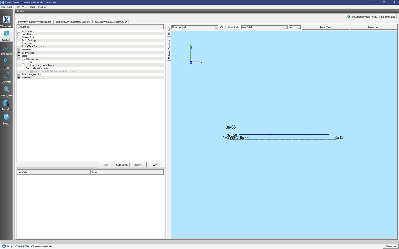
Fig. 239 Choosing the second order accurate, permittivity averaging for the dielectric solver field under Basic Settings and waveguide mode launcher {inactive}.
Running the Pre-run Simulation
After performing the above actions, continue as follows:
Proceed to the Run Window by pressing the Run button in the left column of buttons. If you changed something in the setup, you will be asked to Save. Click Save upon the request to save.
In the left pane :
Set Number of Steps to 1
Set Dump Periodicity to 1.
Check Dump at Time Zero.
Click on the Run button in the upper left corner of the right pane.
You will see the output of the run in the right pane. The run has completed when you see the output, “Engine completed successfully”. This result is shown in Fig. 240.

Fig. 240 Running the simulation for one step to get the permittivity data for the analyzer.
Solving for the Eigenmodes
After performing the above actions, continue as follows:
Proceed to the Analyze Window by clicking the Analyze button on the left.
Select computeWaveguideModes.py and click Open under the list.
Update the analyzer fields accordingly by choosing the corresponding variables under Use Variable :
simulationName: dielectricWaveguideModeCalc
datasetName: invEps
transverseSliceX: PORT_X_INPUT
transverseSliceLY: PORT_YBGN
transverseSliceUY: PORT_YEND
transverseSliceLZ: PORT_ZBGN
transverseSliceUZ: PORT_ZEND
vacWavelength: 1.55e-6
nModes: 1
writeFieldProfile: D
writeFieldNamePrefix: Eigen
modeFileName: port1
Normalize: checked
compMajorC: checked
Overwrite: checked
Click Analyze in the top right corner.
The analyzer will only find guided modes. The results should resemble Fig. 241. We see that the analyzer found the fundamental mode and gives the effective index of the mode under Neff. This parameter is necessary for using the Wave Launcher to launch a unidirectional wave. This value is saved as a parameter as NEFF_FROM_ANALYZER.
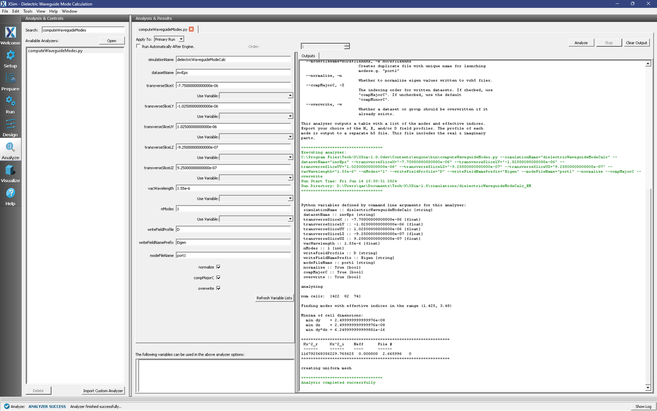
Fig. 241 The analyzer window after a successful run of computeWaveguideModes.py.
Setting up the Main Simulation
After performing the above actions, continue as follows:
Proceed to the Setup Window by pressing the Setup button in the left column of buttons.
Activate the wave launcher
Expand Field Dynamics
Expand CurrentDistributions
Right Click on waveguideModeLauncher0
Left click on Activate
Click on Save and setup in the top right corner.
This setting is shown in Fig. 242.
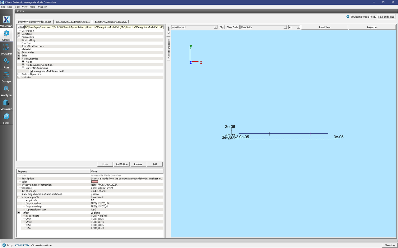
Fig. 242 Activating the wavguide mode launcher.
Running the Main Simulation
After performing the above actions, continue as follows:
Proceed to the Run Window by pressing the Run button in the left column of buttons. You will be asked to Save. Click Save upon the request to save.
In the left pane, click on Reset to Setup Values to run the full simulation which launches this wave down the waveguide.
Check Dump at Time Zero.
Click on the Run button in the upper left corner of the right pane.
You will see the output of the run in the right pane. The run has completed when you see the output, “Engine completed successfully.” This result is shown in Fig. 243.
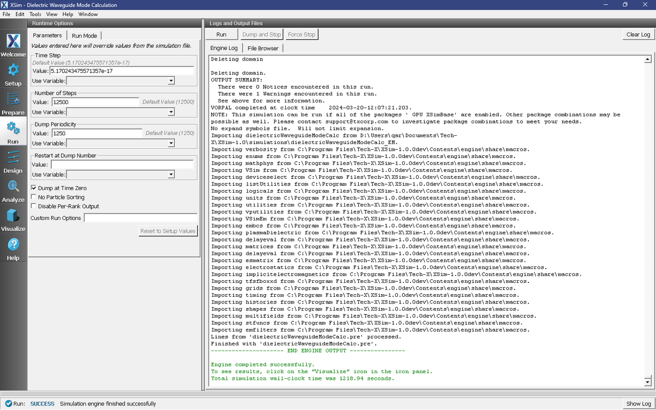
Fig. 243 Running the full simulation which launches this wave down the waveguide.
Visualizing the Results
After performing the above actions, continue as follows:
Proceed to the Visualize Window by pressing the Visualize button in the left column of buttons.
You may need to Reload Data (top right). Visualize an eigenmode by following these steps:
From the Add a Data View dropdown, select Data Overview.
Expand Scalar Data, expand EigenD, and select EigenD_magnitude.
In the Visualization Results window, in the dropdown left of Reset View, select -x to see the mode.
The resulting visualization pane should look like Fig. 244.
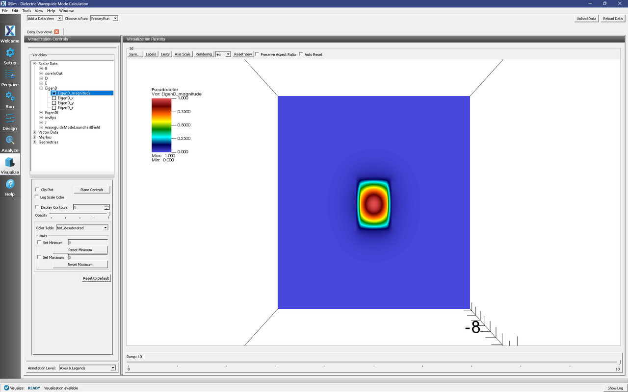
Fig. 244 The visualization pane showing the magnitude of the D field of the fundamental mode.
Analyzing the Results
When designing waveguides, one might be interested in calculating the S parameters and spectral power of the wave traveling down the waveguide. XSim features an analyzer that will compute both of these quantities.
After visualizing the data and making sure the simulation is behaving as expected, proceed to the Analyze Window.
Click on the computeSParamsFromHists.py analyzer to open it and fill in the necessary parameters as follows:
simulationName dielectricWaveguideModeCalc
firstStep: 0
lastStep: 12500
stepOffset: 0
maxWavelength: WAVELENGTH_MAX
minWavelength: WAVELENGTH_MIN
inDirection: 0
inSlabE: slab0_E
inSlabB: slab0_B
inSign: 1
outDirection: 0
outSlabE: slab1_E
outSlabB: slab1_B
outSign: 1
outputFileName : blank
outputSuffix: blank
overwrite: checked
Click Analyze in the top right corner.
The results should resemble Fig. 245
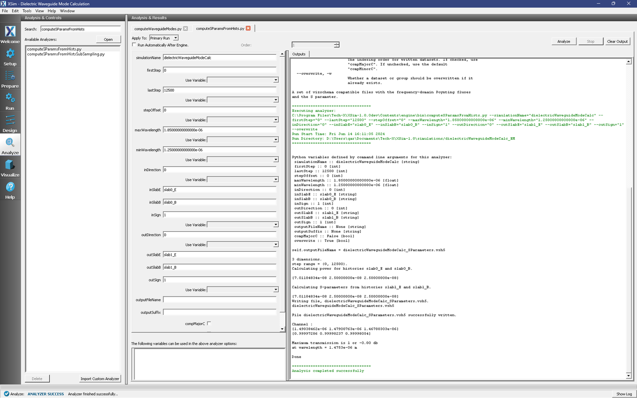
Fig. 245 The analyzer window after a successful run of computeSParamsFromHists.py.
Upon successful completion of the analyzer, proceed to the Visualize tab.
From here, click on the drop down menu called Add a Data View and select 1-D Fields.
To visualize the S-parameters and the input power:
Click Add Curve
Select S_slab1_EAndslab1_B
Click Apply, followed by Ok.
Click on the Add Window button and repeat the same process as before but this time select slab0_EAndslab0_BPower from the drop down menu.
The resulting plots will have the S-parameters per wavelength on top and the spectal input power on the bottom, as in Fig. 246
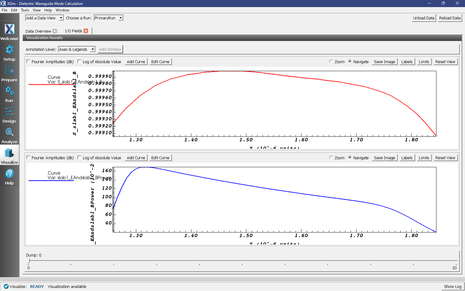
Fig. 246 The visualization window after adding in the plots of the S-parameters and the spectral input power.
Further Experiments
Change the geometry on the Setup window and rerun the simulation and analyzer to see the effects on the modes.
Once you have your desired mode, launch it down the waveguide using the procedure laid out above.
One can run a full convergence study of eigenmode effective indices by changing the resolution in the Setup window and re-running the simulation and mode extraction script. A plot of the effective index as a function of transverse cell area is shown in Fig. 247. The linear relationship shows the second order accuracy of our dielectric algorithms.
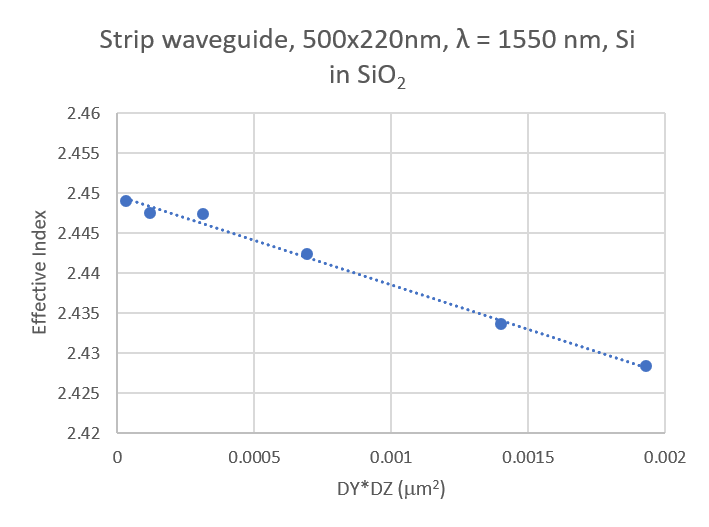
Fig. 247 The effective index as a function of transverse cell area for an eigenmode.