- radiationReaction
Radiation Reaction
This models the radiation reaction process where relativistic electrons spontaneously emit photons when moving in large electric and/or magnetic fields. This process is similar to synchrotron radiation (and is often called nonlinear Compton scattering), but includes a quantum correction since the classical model predicts emission of photons with greater energy than the electron itself under these conditions of \(\gamma \gg 1\) and \(E/E_s=cB/E_s \ll 1\) where \(E_s = m_e^2c^3/(q_e \hbar) \approx 1.32 \times 10^{18}\) V/m is the Schwinger field and \(\gamma\) is the Lorentz factor. This implementation is based on the paper: C. Ridgers et al., J. Comp. Phys. 260 (2014).
The quantum parameter
describes the magnitude of the quantum effects, including the electron momentum loss due to nonlinear Compton scattering. The \(\vec{E}\) and \(\vec{B}\) here are local, instantaneous values at the electron position.
The reaction rate is determined by calculating the cumulative value of the optical depth, \(\tau\), through which the electron has traversed since last emitting. This optical depth is given by
where \(\lambda\) is the approximate rate of emission defined as
In the above equation, \(\alpha_f\) is the fine structure constant, \(\lambda_c\) is the Compton wavelength, \(c\) is the speed of light, and \(h(\eta)\) is the quantum synchrotron function \(F(\eta,\chi)\) integrated over chi. The quantum synchrotron function is defined as
where \(y = 4\chi/(3\eta(\eta-2\chi))\), \(K_n\) are modified Bessel functions of the second kind, and \(\chi\) is related to the resulting photon energy by \(E_{\phi}=h\nu = 2m_ec^2\chi \gamma / \eta\). The function, \(h(\eta)\), has been tabulated for \(\eta \in [10^{-3},10^3]\) where for \(\chi \ge \eta/2\), \(F(\eta,\chi)=0\) and is shown in figure Fig. 623.
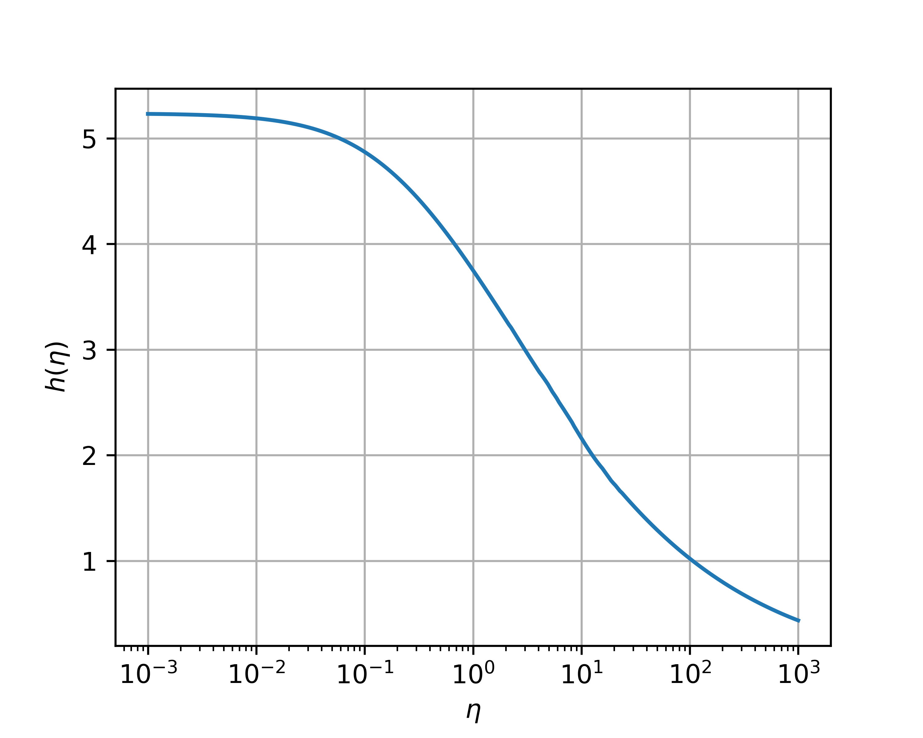
Fig. 623 The function \(h(\eta)\) which determines the emission rate via optical depth calculation.
Therefore, in the Monte Carlo algorithm for this radiation reaction, we only need to calculate the \(\eta\) and \(\gamma\) of the electron, then use these to accumulate the optical depth using simple first order integration, \(\tau(t+\Delta t) = \tau(t) + \lambda(t)\Delta t\). The probability of emission is given by \(p=1-e^{-\tau_{em}}\), and so a threshold value for the optical depth is chosen by inverting this equation and choosing a uniform random number for \(p\in [0,1)\). When \(\tau(t) \ge \tau_{em}\) the emission occurs and the momentum of the resulting photon is subtracted from the electron.
The probability of an electron with quantum parameter \(\eta\) emitting a photon of energy \(\chi\) is given by
This probability distribution has been tabulated and then inverted to obtain \(\chi(\eta,P)\) so that during the simulation a uniformly random \(P\in [0,1)\) is chosen and then bilinear interpolation provides the photon energy \(\chi\) for the given electron \(\eta\). These functions, \(P(\eta,\chi)\) and \(\chi(\eta,P)\), are shown in figure Fig. 624.
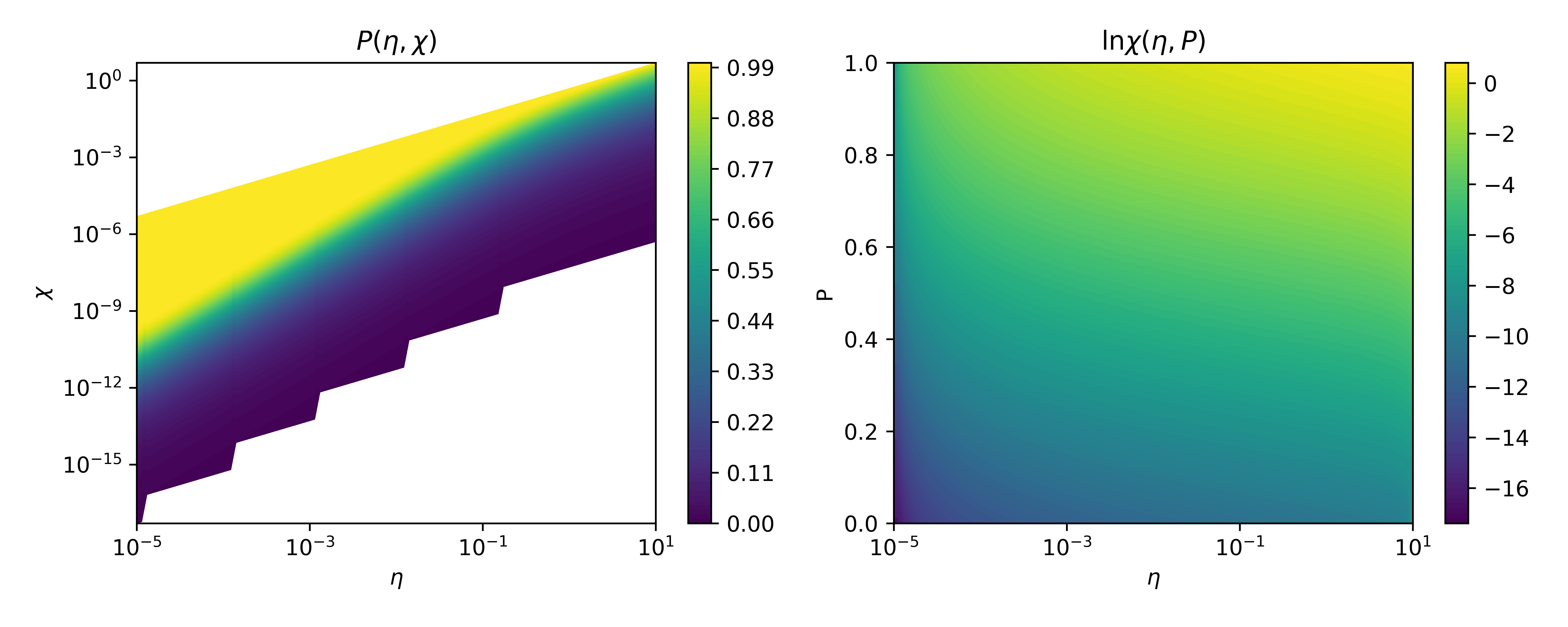
Fig. 624 Plots of \(P(\eta,\chi)\) and the inverted \(\ln \chi(\eta,P)\) used for sampling the emitted photon energy.
Note
Specific RxnRateCalculator and RxnProductGenerator must be paired for radiation reaction. Also, the species must be relBorisRad, relBorisRadVW, relBorisRadCyl, or relBorisRadCylVW so that t he optical depth can be tracked for each particle.
Any RxnProcess Block block which points to a
productGenerator of kind = radiationReaction should have the
Reactants and Products in the order:
reactants = [electrons E B]
products = [electrons (photon)]
The optional photon in the product block allows the production of photons from this process. The photon must be of kind=freeRelVW and it will store the energy of the photon as the weight, and the number of physical photons represented by the emission as 100 times the relativistic gamma. One can place an AbsAndSave boundary over the entire domain and the emitted photons will be immediately absorbed upon emission with their information saved and accessible via the speciesAbsPtclData2. Alternatively, one can let these photons propagate freely through the domain, but since this is more expensive it is only recommended if one cares about their trajectories.
Validation
Three test cases are given in the Ridgers (2014) paper, and we have validated our implementation for these same cases. These are:
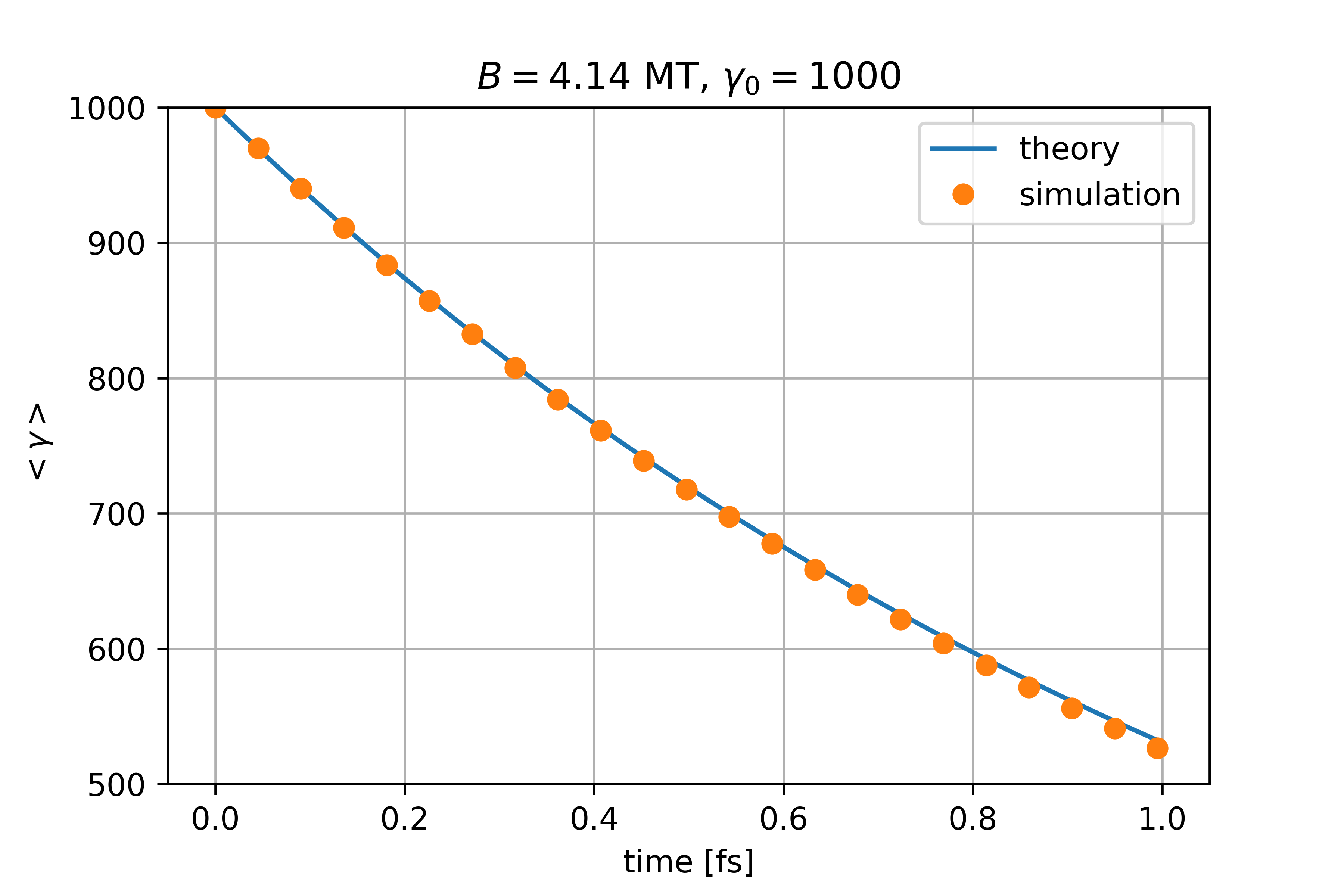
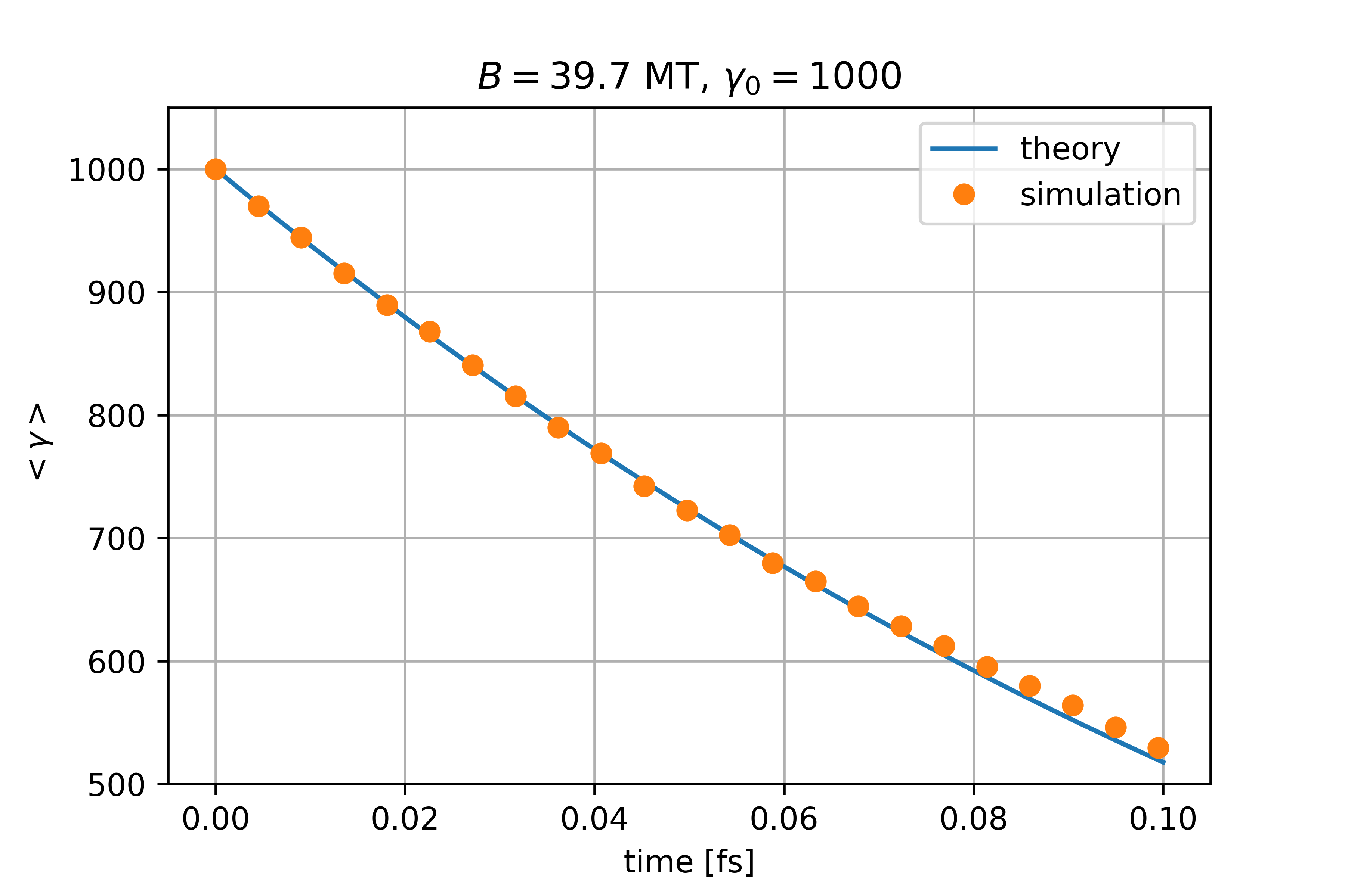
1. Electrons moving in large \(B\) field with \(\gamma_0=1000\) and \(\eta=1\)
2. Electrons moving in larger \(B\) field with \(\gamma_0=1000\) and \(\eta=9\)
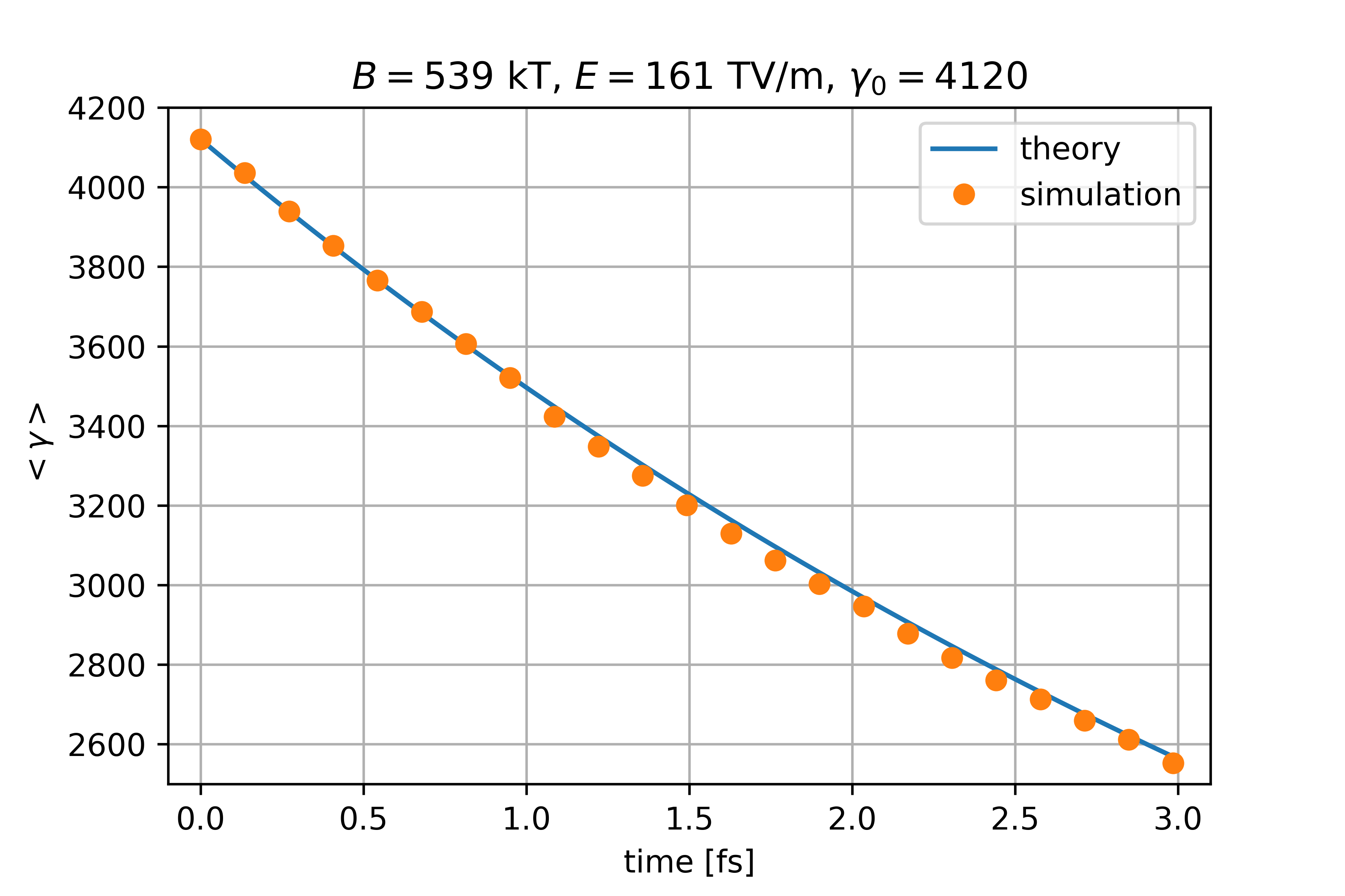
3. Electrons counter-propagating in a circularly polarized EM wave with \(\gamma_0=4120\) and \(\eta=1\)
These simple situations have analytic solutions, and we find agreement between the theory and our simulation results as seen in the figures below:
reactionRate Attributes
- kind (string, required)
Use the string
radiationReaction
reactionProductGenerator Attributes
- kind (string, required)
Use the string
radiationReaction
Example radiationReaction Input File Blocks
<RxnProcess radRxn>
  kind = collisionProcess
  rxnPhysics = radRxnPhys
  reactants = [electrons multiField.E multiField.B]
  products = [electrons]
  # randomSeed = 1000
</RxnProcess>

<RxnPhysics radRxnPhys>
  kind = generalCollision
  <RxnRate rxnRate>
    kind = radiationReaction
  </RxnRate>
  <RxnProductGenerator productGenerator>
    kind = radiationReaction
  </RxnProductGenerator>
</RxnPhysics>