Reactions Introduction
The following pages of documentation provide details of setting up interactions between kinetically modeled particle species, background fluids/gases, or any combination of particles and fluids in the “Reactions” framework. For a list of supported interactions see RxnProductGenerator Sub-Block. A sample of a complete set of blocks that adds a electron attachment process to a simulation is included at the end of this page. For a user-centric description of this set of blocks see User Guide: Simulation Concepts: Collisions in the user guide.
Anisotropy
For some reactions the option is available to specify the anisotropy of the product distribution. This is specified in the range [-1,1] where 0 is isotropic, -1 results in back scatter, and 1 results in forward scatter. Since anisotropy is a collective behavior, each reaction will not necessarily satisfy this qualitative criteria, but overall the reactions will result in scattering angles as shown in Fig. 619.
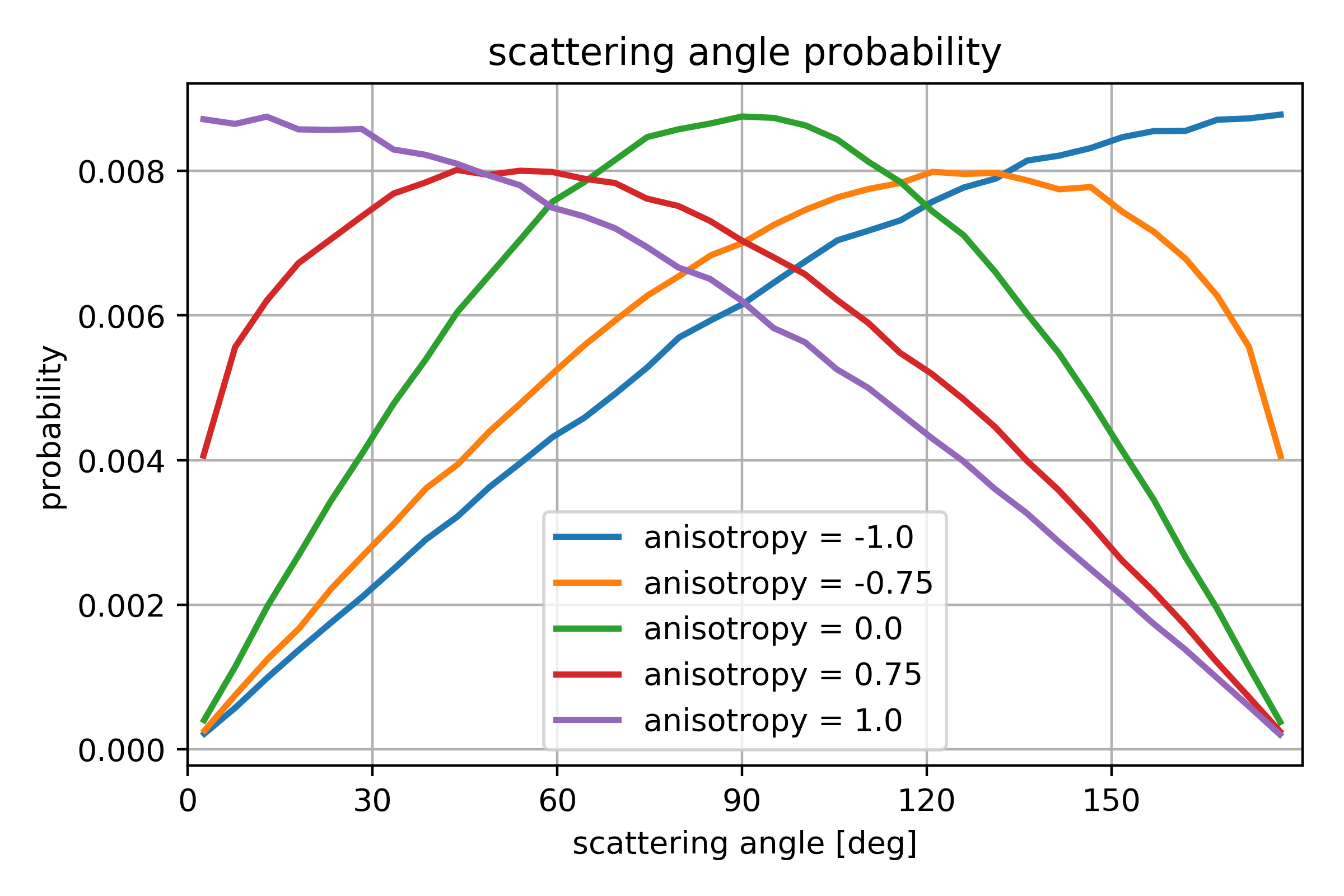
Fig. 619 Angular distribution for several choices of anisotropy
For a single reaction, the scattering angle is chosen using a random number \(r \in \left[0,1 \right)\) and the following equation:
where \(a\) is
where \(A\) is the anisotropy value set by the user in a code block.
If \(a\) is negative, we use the absolute value to calculate theta but then reverse the center of momentum velocity of the particles during the calculation of the collision vector.
Reactions Algorithm
Consider a simulation cell with \(N\) particles of one species interacting with \(M\) particles of another. The total number of combinations of possible reactions is then
A set of \(N_R\) reaction pairs could then be generated, resulting in a total number of reactions occurring given by
where \(P_{rxn}\) is the individual probability of each reaction pair colliding, which is likely different for each pair. Therefore, the average probability times the total possible reaction pairs gives the total number of reactions that will occur. This requires calculating the reaction probability of \(NM\) reaction pairs, which is computationally expensive.
Null Probability
It would be nice to reduce the number of reaction pairs chosen to increase computational efficiency, while maintaining accuracy. The null probability provides the answer here. It is calculated and used as a way to sub-sample the reaction pairs, while proportionally increasing their reaction probability. This should result in the same overall number of reactions as if the full, brute-force method were used. Null probability is defined as
where \(\sigma\) is the cross section of the reaction process, \(v\) is the relative velocity of the particles involved, \(W\) is the weight of the particle (number of physical particles per macro particle), \(\Delta t\) is the time step, and \(V\) is the volume of the simulation cell. This denotes the maximum probability in the cell and is used to normalize the reaction probability such that the reaction pair with the highest probability will then have 100% chance to occur. The number of reaction pairs chosen to potentially collide, then is
Thus, the reaction probability for each chosen reaction pair reaction is
Using this probability along with the number of reaction pairs, we can calculate how many reactions occur.
We see that, assuming the subset of particles we chose has the same average reaction probability as the full set, the number of reactions that occur matches exactly what should occur in the full method which is calculated in the first equation for \(N_{occ}\) above.
This has the desired effect, but there are some intricacies that need addressing.
Caveats
We have decided to only have each particle interact once per time step, so each particle can only interact with one other particle. This can be accomplished in one of two ways, though only one will give the correct number of reactions.
In the case where \(N_{pairs}\) is greater than the lesser of \(M\) and \(N\), a single particle must appear more than once in the list of reaction pairs. The question then, is what to do in this case.
Remove Duplicates After Reactions
The original implementation involved generating a full list of \(NMP_{null}\) pairs, even if there a single particle appears multiple times in this list. Then we go through and determine which reaction pairs actually collide. We then remove any duplicates from the list of collision pairs that actually collide. The theoretical number of reactions that occur should then be correct with \(N_{occ} = NM\left< P_{rxn} \right>\). However, in the case where duplicates are removed, the number of occurring reactions is artificially lowered from this true reaction rate.
Never Include Duplicates
If we instead generate a list of reaction pairs such that there are no duplicates, the number of pairs is given by
We will assume that \(N \le M\) from this point on, reducing the above equation to
This leaves two cases to explore. The case where \(N_{pairs} = NMP_{null}\) has already been described in section 2 as the standard case for the use of null collision probability.
However, if \(N_{pairs} = N\), we must then redefine the null probability to have the correct number of reactions occur. This is because the null probability is the ratio of the number of reaction pairs chosen to the total number of possible reaction pairs, as stated in the equation \(N_{pairs} = N_R P_{null}\) (see equation above).
By adjusting the null probability to be the true number of reaction pairs chosen over the total possible, the number of reactions that occurs remains accurate:
This second method of never including duplicates is thus more accurate than the first where duplicates are removed; however, both have the same limitation. When \(N_{occ} > N\) (ie. more reactions should occur than we have particles in the cell), we find that \(P_{rxn} > P_{null}\), which can lead to an underestimation of the reaction rate. For such a situation, the time step should be lowered to maintain \(N_{occ} \le N\).
Example of a “Fully-Assembled” Set of Reactions Code Blocks
<RxnProcessSettings RxnProcessSettings>
  updateOrder = random
  updatePeriod = [ 1 ]
</RxnProcessSettings>

<Reactant neutralArgonReactant>
  kind = neutralGas
  neutralGasName = neutralArgon
</Reactant>

<Reactant electronsReactant>
  kind = particle
  ptclSpeciesName = electrons
</Reactant>

<Reactant ArMinusReactant>
  kind = particle
  ptclSpeciesName = ArMinus
</Reactant>

<RxnProcess electronAttachmentParticlesRXN0>
  kind = collisionProcess
  reactants = [neutralArgonReactant electronsReactant]
  products = [ArMinusReactant]
  rxnPhysics = electronAttachmentParticlesRXN0electronAttachment
  verbosity = 127
</RxnProcess>

<RxnPhysics electronAttachmentParticlesRXN0electronAttachment>
  kind = generalCollision
  <RxnRate rxnRate>
    kind = twoColumnFile
    crossSectionVariable = velocity
    file = 2ColumnData.dat
  </RxnRate>

  <RxnProductGenerator productGenerator>
    kind = electronAttachment
    thresholdEnergy = 1.0
  </RxnProductGenerator>
</RxnPhysics>