S-Matrix of Box Cavity (sMatrix.sdf)
Keywords:
- electromagnetics, sMatrix
Problem description
A common measurement made on a 2-port RF device is reflection and transmission of an RF signal, for either a single frequency, or for a range of frequencies. This measurement results in the Scattering-Matrix, or S-Matrix, whose elements S11 and S21 are the reflected and transmitted signal for unit input at Port 1. VSim provides the capability to simulate these S-Matrix parameters for arbitrarily complex devices connected to waveguides propagating TE, TM, and TEM modes. To demonstrate this capability, we show in this example how to measure S11 and S21 in a dual-mode cavity filter, connected to a WR-90 waveguide, with the narrow-band band-pass tuned to pass frequencies between 9.95 and 10.05 GHz.
The Dual Mode Cavity Filter operates by coupling the TE01 waveguide mode into the two nearly degenerate TE102 and TE201 modes of the cavity, since the length of the cavity is very close to its width. The differences in these values, along with the symmetry breaking along the waveguide axis, determine the frequency separation of the two modes. This separation is what gives the filter finite-bandwidth since frequencies between these modes are passed, and frequencies above or below the modes are rejected. A pole in the transmitted signal just below the band contributes to sharpness of the band’s lower edge, but this pole moves easily to the upper frequency edge with small adjustments to the cavity dimension parameters, and the user is encouraged to experiment in finding optimal placement of this pole. Some relevant parameters are shown in Fig. 381.
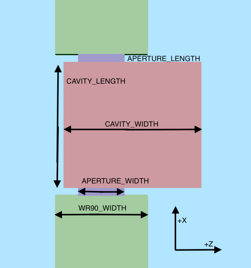
Fig. 381 Some relevant parameters for the S-Matrix Box Cavity example.
Opening the Simulation
The Scattering Matrix example is accessed from within VSimComposer by the following actions:
Select the New → From Example… menu item in the File menu.
In the resulting Examples window expand the VSim for Vacuum Electronics option.
Expand the Cavities and Waveguides option.
Select “S-Matrix of Box Cavity” and press the Choose button.
In the resulting dialog, create a New Folder if desired, and press the Save button to create a copy of this example.
The Setup Window is now shown with the waveguide in the 3D View. Fig. 382.
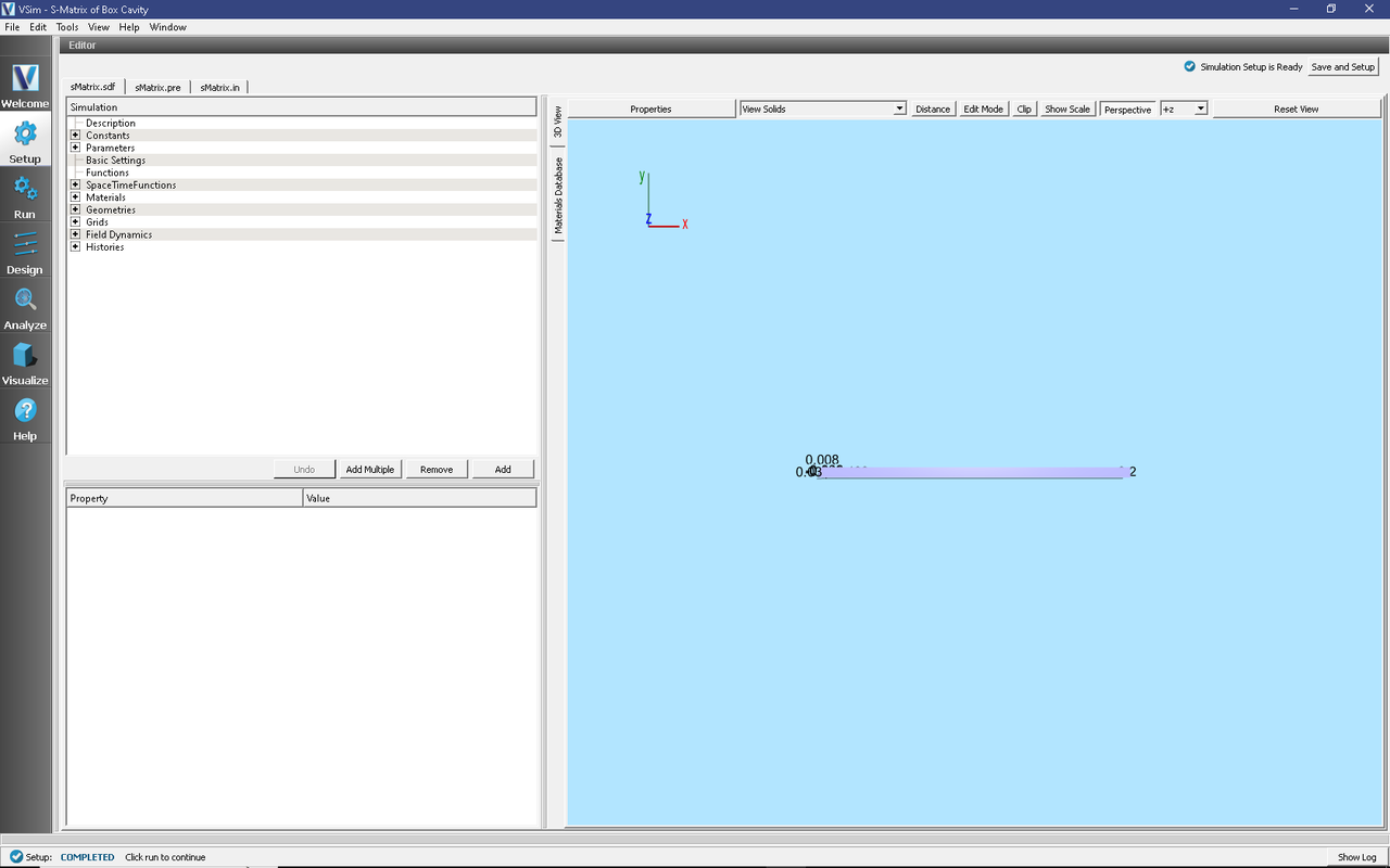
Fig. 382 Setup Window for the Scattering Matrix example.
Simulation Properties
The simulation geometry consists of a standard WR-90 rectangular waveguide with the filter cavity (also referred to as the Device-Under-Test (DUT) in this writeup) in the center. A planar antenna in the waveguide, near the DUT, launches the incident wave while allowing reflected signals to pass through into the waveguide behind it. The antenna is constructed of two planar current sources with each current source one cell thick in the x-direction and directly adjacent to each other along x. The amplitudes and phases of the current sources are tuned so that the electric and magnetic fields which launch in the -x direction cancel whereas in the +x direction, the fields add to a non-trivial value. The waveguide ends are terminated in gradual absorbing layers with negligible reflection, and the reflected and transmitted signals are measured just in front of these absorbers.
This example is parameterized in the waveguide and DUT geometry specification, allowing for easy modification to either. Thus this example is effectively a template for an S-Matrix simulation of any device. The time histories of voltage signals used to measure S11 and S21 are also built in and automated for easy substitution. Furthermore, these signals are easily turned into S11 and S21 frequency variation curves using the standard “Fourier Amplitudes” capabilities in VSimComposer, or if single frequency, then the S11 and S21 values are just the amplitudes of the signals.
The x axis is the axial direction of the waveguide, with the parameters WAVEGUIDE_LENGTH, APERTURE_LENGTH, and CAVITY_LENGTH controlling the lengths of each component. These parameters are also used to control the position of each component, allowing a change to one of them to properly adjust the component positions.
The height (Y axis) of each component is standardized to the parameter WR90_HEIGHT, and centered around the Y axis.
The waveguide and aperture widths are centered around the Z axis, while the cavity is not.
The excited mode is the standard lowest mode, TE01, and in particular note that for this mode, the Ez component of the field is zero. The spatial profile of the current source is consistent with the TE01 mode. Since we are launching a TE01 mode, the perpendicular component of the electric field is 0 at the boundaries. Because the larger waveguide dimension is along z the lowest order mode coincides with the y-component of the electric field being excited. Therefore the function “waveguideEyProfile” is the spatial function used in the current source in order to launch the desired waveguide mode.
Running the simulation
After performing the above actions, continue as follows:
Proceed to the Run Window by pressing the Run button in the left column of buttons.
To run the file, click on the Run button in the upper left corner of the right pane. You will see the output of the run in the right pane. The run has completed when you see the output, “Engine completed successfully.” This is shown in the window below.
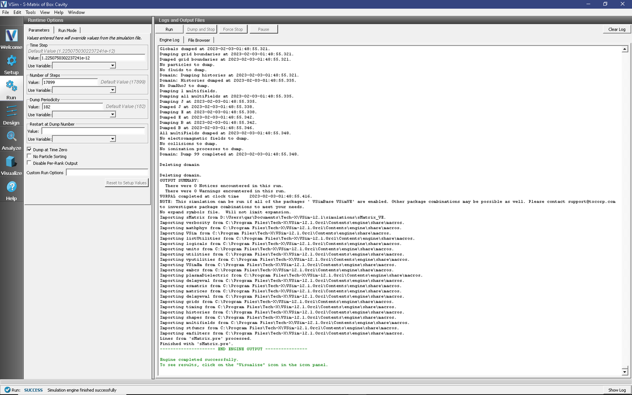
Fig. 383 The Run Window at the end of execution.
This example is more sophisticated than some of the others, in that successful determination of S-Matrix parameters is not the result of a single run, but rather a result of a procedure involving several runs. This includes at least one Calibration Run, and at least one Data Run to determine S11 and S21. Below we discuss in detail some of the features of this example.
Frequency Band vs. Single Frequency
The user may choose whether to compute a single-frequency value of the S-Matrix parameters, or to compute the variation of the parameters as a function of frequency across a user specified frequency band. The constant, FREQCENTER, specifies either the single frequency or the center frequency of the band. The constant, FREQBANDWIDTH, provides the bandwidth or is set to 0 if a single-frequency simulation is desired.
With a single frequency simulation, the constant, NUMBEROFCYCLESTODRIVE, should be large enough to ensure that the S11 and S21 histories reach a steady amplitude. The History data view can be used to obtain the S-Matrix value, which is just the amplitude of the signal.
With a finite frequency band, the same constant, NUMBEROFCYCLESTODRIVE, can be adjusted upward to increase the detail and sharpness of the S-Matrix variation with frequency. In particular, increasing NUMBEROFCYCLESTODRIVE causes the FFT of the S11 and S21 histories to attain a sharper cutoff at FREQHI and FREQLO. The constant, NUMBEROFCYCLESTOCOAST, may also need to be adjusted upward if the DUT contains internal mode oscillation of large Q (quality) factor. This variable needs to be large enough so that the signal histories have decreased to a negligible value (10-4, relative to maximum) by the end of the simulation. The FFT button in the History data view is then used to give the S-Matrix variation with frequency, with the plot’s Y-axis units being dB. Be aware that it is usually necessary to zoom in significantly on this plot in order to see the frequency band of interest.
Finally, in both these cases, only the amplitude of the complex-valued S-Matrix parameters can be obtained with VSimComposer. More sophisticated post-processing (not covered in this example) is needed in order to get the phase information.
Calibration Run
The Calibration Run is done first, and the user must ensure that in the geometries, only the material of the object myCalibrationWaveguide is set to PEC, i.e., ensuring the material of the object myWaveguideAndDUT is set to empty. In the Calibration Run, the DUT is automatically omitted and replaced with a continuation of the waveguide, so that this is a near trivial simulation of a straight length of waveguide that should have effectively 100% transmission. The calibration run serves two very important purposes:
To ensure that there is negligible (below 1% amplitude, -40 dB) reflected voltage (S11). If the reflection is too high it indicates that either the absorbing boundaries (MAL’s) are not working well enough, or that the waveguide’s “modeProfile” description is not accurate enough, and/or that there is not enough grid resolution. To decrease reflections at the MAL boundaries, you can decrease the “damping factor” in the MAL boundary condition. If you do this, you may need to increase the length of the MAL. Another potential issue is the value of TRISE, which is the length of time over which the current source is turned in the single frequency runs. Increasing TRISE could lead to a better measure of S11 and S21.
To adjust the DRIVENORMALIZATION constant, which runs in proportion to observed transmitted voltage (S21), so that the next time the calibration run is done, the transmitted voltage (S21) will be exactly unit amplitude (single frequency) or zero dB (across frequency band). For example, if the first Calibration Run shows an amplitude of 0.667 for S21, change DRIVENORMALIZATION to 1.5 times its present value for the next Calibration Run, since 1/0.667 = 1.5.
Changing center frequency, or any waveguide parameter, or even the nominal cell size, will require re-calibration. If not sure, always recalibrate, when changing a parameter.
Data Run
Once the Calibration Run is successful at achieving unit transmission with negligible reflection, the Data Run is then done. The user should ensure that only the material of the object myWaveguideAndDUT is set to PEC, i.e., ensuring the material of the object metalMinuscalibrationWaveguide is set to empty.
Visualizing the results
After performing the above actions, continue as follows:
Proceed to the Visualize Window by pressing the Visualize button in the left column of buttons.
The S-Matrix results are shown by adding a History data view. Once the history graphs are displayed check Fourier Amplitudes to get an FFT of the data. To look at the results from 8 to 12 GHz, click Limits in the upper right corner of each graph and set the X-axis lower limit to 6e9, and upper limit to 14e9.
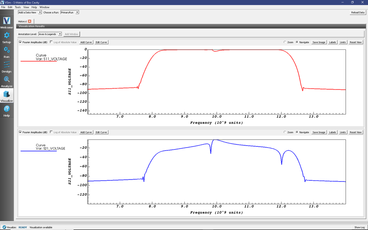
Fig. 384 Fourier transforms of the histories S11_Voltage and S21_Voltage as a function of frequency (in GHz).
Further Experiments
Experiment with finding optimal placement of the pole in the transmitted signal.